The ACF or autocorrelation function is a measure of the correlation between a time series and its lagged values. People talk about the memory and memorylessness of distribution and autoregressive processes. But these are often intuitively understood rather than rigorously defined. It turns out that while this mental model of memory in time series etc is useful, it will only get us so far and eventually may become counterproductive. Unfortunately I cannot give you a definite answer of how to map the mental model to mathematical rigor. The best I can do is point out that there are a number of formal definitions that seem to map to our intuitive understanding of memory.
ACF, Autocorrelation function (ACF),
PACF, Partial autocorrelation function (PACF),
Stationarity,
Strict stationarity,
Weak stationarity,
Order of a TS process like p in AR(p) and q in MA(q),
Periodicity, and
Pseudo-periodicity a nemesis of stationarity.
These are the cognates of intuitive memory that I learned in the coursera Bayesian specialization. Looking further a field, there is the Markov property, which is a formal definition of memorylessness, where we say that a process is Markovian if the future is independent of the past given the present. However when it comes to more general models like NDLMs
All this brings us to the first problem, This is an ACF derivation from assumption of stationary for AR(1) model. However we are in the part of the book that is concerned with generalities and so the next problem set will delve deeper in AR(P) models and here we look at the AR(1) which is the simplest example and amenable to pen and paper analysis.
Exercise 103.1 Show that the autocorrelation function (ACF) of an AR(1) is \rho(h) = \phi^{\mid h\mid } \qquad h = 0, \pm 1, \pm 2, \ldots
where:
the process parameter \phi with |\phi| <1,
with innovation \varepsilon \sim \mathcal{N}(0, v)
and \rho(\varepsilon_t, \varepsilon_s)=0 i.e. uncorrelated innovations.
The autocorrelation function (ACF) is given by:
\begin{aligned}
\rho(h) &= \frac{\mathrm{Cov}(Y_t, Y_{t+h})}{\sigma^2} \\
&= \frac{\phi^{|h|} \sigma^2}{\sigma^2} \\
&= \phi^{|h|}
\end{aligned}
Assume that v is known. Find the MAP estimator of \phi under a uniform prior p(\phi) = \mathcal{U}(\phi\mid −1, 1) for
the conditional likelihood and
the unconditional likelihoods.
Comment: We talk about three types of point estimates in Bayesian analysis. They are:
Maximum Likelihood Estimation (MLE): This is the most common method, where we find the parameter values that maximize the likelihood function. This is actually the frequentist approach, as it does not incorporate prior beliefs about the parameters. We like to use it as it can show us what a frequentist might report as a point estimate, and we can use it as a baseline in Bayesian analysis.
MAP Estimation: The Maximum A Posteriori (MAP) estimate is the mode of the posterior distribution and can be seen as a compromise between MLE and Bayesian estimation. In this case, we also need a prior and we can use a reference prior, a uniform prior or a conjugate prior.
Least Squares Estimation: This is a special case of MLE where we minimize the sum of squared residuals. It is often arises when we can look at a model as a linear regression models.
So although as Bayesians we are less concerned with point estimates, questions about these may come out of the blue, and we should be able to not only answer them, but also understand the differences between them and justify our choice of prior if we use MAP estimation.
TipSolution:
Conditional likelihood
The conditional log‐likelihood (conditioning on y_1) is
\ell_c(\phi,v)
= -\frac{T-1}{2}\log v - \frac{1}{2v}\sum_{t=2}^T (y_t - \phi y_{t-1})^2.
With a flat prior on |\phi|<1, the posterior is proportional to the likelihood (conditional or unconditional) on that interval. Hence the MAP equals the corresponding MLE, provided it lies in (-1,1); otherwise, the posterior mode is at the nearest boundary \phi=\pm1. Specifically:
Show that under the reference analysis discussed in (Prado, Ferreira, and West 2023, sec. 1.5.3) where we assume a prior p(\beta , v) \propto 1/v The corresponding posterior density is p(\beta, v\mid y, F) \propto p(y\mid F, \beta, v)/v
where c(n,p) = \frac{\Gamma(n/2)}{[\Gamma((n − p)/2)(s^2 \pi(n − p))^{p/2}]},
The marginal density:
p(y\mid F) = \int p(y\mid F, \beta , v)p(\beta , v)d\beta dv
Comment: I think We mentioned reference analysis in course two of the specialization but I assumed a base line model. This looks pretty scary at first glance.
However, I recall seeing Student t’s t-distribution appearing out of the blue in a couple of places, could it be due to the reference analysis i.e. introducing a Jeffreys prior? I think so!
TipSolution:
Let y\in\mathbb R^{n}, F\in\mathbb R^{p\times n}, \beta\in\mathbb R^{p}, model y\mid\beta,v \sim \mathcal N(F^\top\beta, v I_n), and prior p(\beta,v)\propto 1/v(Prado, Ferreira, and West 2023, sec. 1.5.3)
Exercise 103.4 Show that the distributions of (\phi\mid y, F) and (v\mid y, F) obtained for the AR(1) reference analysis using the conditional likelihood are those given in (Prado, Ferreira, and West 2023 Example 1.6),
i.e. Reference analysis in the AR(1) model.
Assume the AR(1) model :
y = (y_2 , \ldots , y_T )^\top , F =(_y1 , \ldots , y_{T −1} ) and
the reference prior p(\phi, v) \propto 1/v
(\phi\mid y, F) \sim t_{(T −2)} (m,\frac{C}{T − 2}),
where m = \frac{ \sum_{t=2}^T y_t y_{t−1}}{\sum_{t=1}^{T-1} y^2} and C = \frac{\sum_{t=2}^T y_t^2 {\sum_{t=2}^{T} y_t-1}^2 - \sum_{t=2}^T (y_t y_{t−1})^2}{\sum_{t=1}^{T-1} y_t^2}.
where m = \frac{1}{T − 1} \sum_{t=2}^T y_t y_{t−1} and SSE(\phi) = \sum_{t=2}^T (y_t − m y_{t−1})^2.
Exercise 103.5
Show that the expressions for the distributions of (y\mid F, v), (v\mid y, F), and (\beta \mid y, F) under the conjugate analysis in (Prado, Ferreira, and West 2023, sec. 1.5.3) are those given on page 24.
Exercise 103.6 Show that the distributions of (\phi \mid \mathbf{y}, \mathbf{F}) and (v \mid \mathbf{y}, \mathbf{F}) obtained for the AR(1) conjugate analysis using the conditional likelihood are those given in Example 1.7.
Assume we choose a prior of the form : \phi|v \sim \mathcal{N} (0, v) and v \sim \mathcal{IG}(n0 /2, d0 /2), with n0 and d0 known.
Exercise 103.7 Consider the following models:
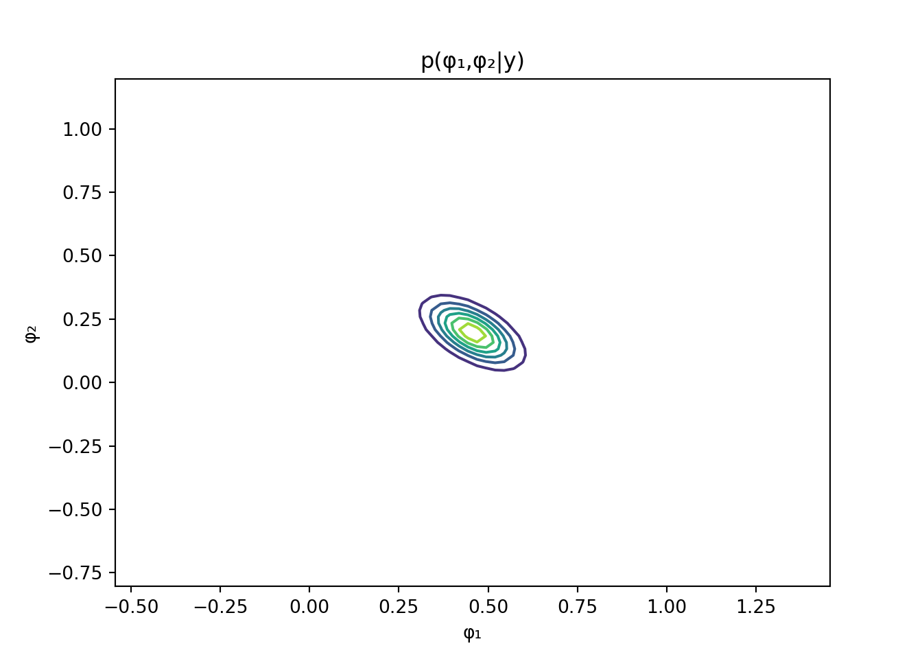
y_t= \phi_1 y_{t−1} + \phi_2 y_{t−2} + \varepsilon_t \qquad (1.26)
\tag{103.1}
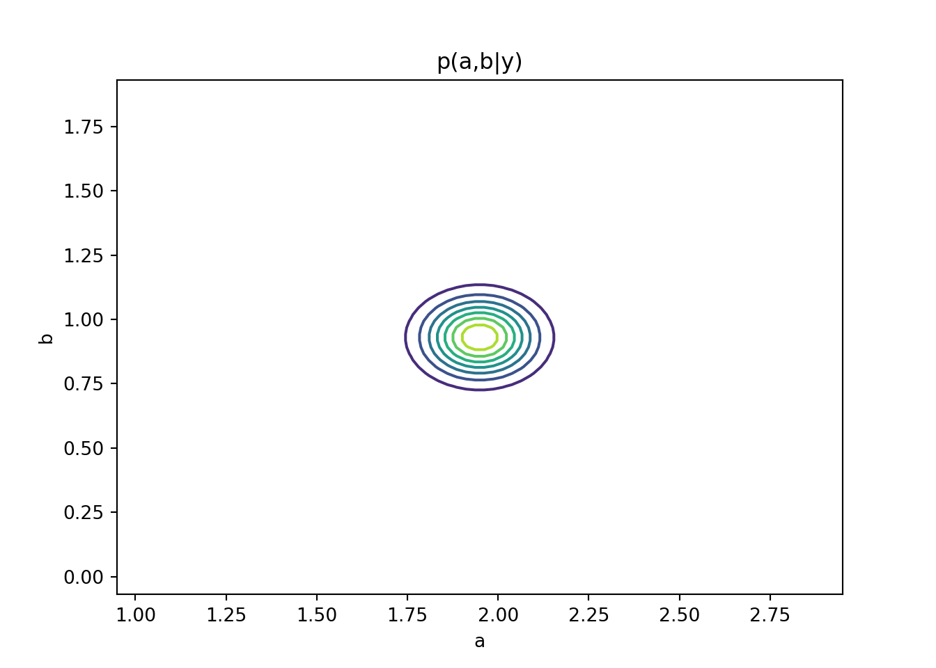
y_t= a \cos(2\pi \omega_0 t) + b \sin(2\pi \omega_0 t) + \varepsilon_t \qquad (1.27)
\tag{103.2}
with
\varepsilon_t \sim \mathcal{N} (0, v)
and \omega_0 > 0 fixed.
Sample T = 200 observations from each model using your favorite choice of the parameters. Make sure your choice of (\phi_1 , \phi_2 ) in model (Equation 103.1) lies in the stationary region. That is, choose \phi_1 and \phi_2 such that −1 < \phi_2 < 1, \phi_1 < 1 − \phi_2, and \phi_1 > \phi_2 − 1.
Find the MAP estimators of the model parameters under the reference prior. Again, use the conditional likelihood for model (Equation 103.1).
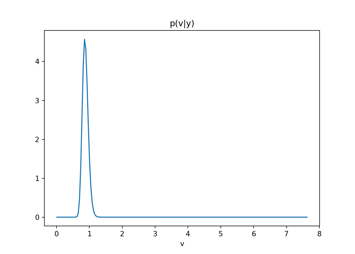
Sketch p(v\mid y, F) and p(\phi_1 , \phi_2 \mid y, F) for model (Equation 103.1).
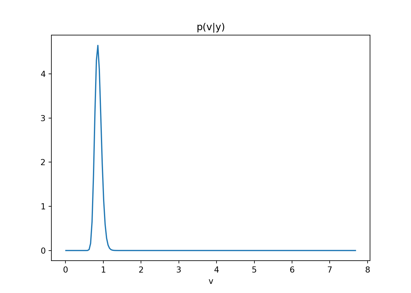
Sketch p(a, b\mid y, F) and p(v\mid y, F) for model (Equation 103.2).
Perform a conjugate Bayesian analysis, i.e., repeat 3-4 assuming conjugate prior distributions in both models. Study the sensitivity of the posterior distributions to the choice of the hyperparameters in the prior.
TipSolution:
# Exercise 1.7-7: AR(2) and Sinusoidal Models########################################################### This script solves the six tasks in Exercise 1.7-7:# 1. Simulate T=200 observations from an AR(2) model and a sinusoidal model.# 2. Compute MLEs of parameters using conditional likelihood for AR(2) and OLS for sinusoid.# 3. Compute MAP estimators under the reference prior p(φ,v) ∝ 1/v.# 4. Sketch posterior p(v|y,F) and p(φ₁,φ₂|y,F) for AR(2).# 5. Sketch posterior p(a,b|y,F) and p(v|y,F) for the sinusoidal model.# 6. Perform conjugate Bayesian analysis for both models and study sensitivity.import numpy as npimport matplotlib.pyplot as pltfrom scipy.stats import invgamma############################## Part 1: Simulation#############################def simulate_ar2(phi, sigma2, T, seed=None):""" Generate AR(2) data: y_t = φ₁ y_{t−1} + φ₂ y_{t−2} + ε_t, ε_t∼N(0,σ²). Returns array of length T. """if seed isnotNone: np.random.seed(seed) y = np.zeros(T) eps = np.random.normal(0, np.sqrt(sigma2), size=T)for t inrange(2, T): y[t] = phi[0]*y[t-1] + phi[1]*y[t-2] + eps[t]return ydef simulate_sin(ab, omega0, sigma2, T, seed=None):""" Generate sinusoidal data: y_t = a cos(2π ω₀ t) + b sin(2π ω₀ t) + ε_t. Returns time index and observations. """if seed isnotNone: np.random.seed(seed) t = np.arange(1, T+1) a, b = ab deterministic = a*np.cos(2*np.pi*omega0*t) + b*np.sin(2*np.pi*omega0*t) noise = np.random.normal(0, np.sqrt(sigma2), size=T)return t, deterministic + noise############################## Part 2: Maximum Likelihood#############################def mle_ar2(y):""" MLE for AR(2) via OLS on y[2:] ~ y[1:-1], y[:-2]. Returns φ̂ = [φ₁,φ₂], σ̂². """ Y = y[2:] X = np.column_stack([y[1:-1], y[:-2]]) phi_hat, *_ = np.linalg.lstsq(X, Y, rcond=None) resid = Y - X.dot(phi_hat) sigma2_hat = np.mean(resid**2)return phi_hat, sigma2_hatdef mle_sin(y, omega0):""" MLE for sinusoid via OLS on y ~ cos(2πω₀t), sin(2πω₀t). Returns [â,b̂], σ̂². """ T =len(y) t = np.arange(1, T+1) X = np.column_stack([ np.cos(2*np.pi*omega0*t), np.sin(2*np.pi*omega0*t) ]) ab_hat, *_ = np.linalg.lstsq(X, y, rcond=None) resid = y - X.dot(ab_hat) sigma2_hat = np.mean(resid**2)return ab_hat, sigma2_hat############################## Part 3: MAP under Reference Prior#############################def map_ref_ar2(y):""" MAP under p(φ,v) ∝ 1/v for AR(2). φ̂ same as MLE, v̂ = (SSE/2)/(n/2 + 1). """ Y = y[2:]; X = np.column_stack([y[1:-1], y[:-2]]) phi_mle, sigma2_mle = mle_ar2(y) resid = Y - X.dot(phi_mle) n =len(Y) SSE = resid.dot(resid) alpha, beta = n/2, SSE/2 v_map = beta/(alpha +1)return phi_mle, v_mapdef map_ref_sin(y, omega0):""" MAP under p(a,b,v) ∝ 1/v for sinusoid. (a,b)̂ same as MLE, v̂ MAP as above. """ ab_hat, _ = mle_sin(y, omega0) t = np.arange(1, len(y)+1) X = np.column_stack([ np.cos(2*np.pi*omega0*t), np.sin(2*np.pi*omega0*t) ]) resid = y - X.dot(ab_hat) n =len(y) SSE = resid.dot(resid) alpha, beta = n/2, SSE/2 v_map = beta/(alpha +1)return ab_hat, v_map############################## Part 4 & 5: Posterior Sketches#############################def plot_posteriors_ar2(phi_map, y):""" Plot posterior contours for φ and density for v under reference prior. """ Y = y[2:]; X = np.column_stack([y[1:-1], y[:-2]]) phi_hat = phi_map A_inv = np.linalg.inv(X.T.dot(X))# φ posterior: approx N(phi_hat, v*inv(X'X)) scaled out v grid = np.linspace(-1,1,80) P1,P2 = np.meshgrid(grid+phi_hat[0], grid+phi_hat[1]) invA = np.linalg.inv(A_inv) norm =1/(2*np.pi*np.sqrt(np.linalg.det(A_inv))) Z = norm * np.exp(-0.5*( invA[0,0]*(P1-phi_hat[0])**2+2*invA[0,1]*(P1-phi_hat[0])*(P2-phi_hat[1]) + invA[1,1]*(P2-phi_hat[1])**2 )) plt.contour(P1,P2,Z) plt.title("p(φ₁,φ₂|y)"); plt.xlabel('φ₁'); plt.ylabel('φ₂') plt.show() resid = Y - X.dot(phi_hat) n =len(Y); SSE = resid.dot(resid) alpha,beta = n/2, SSE/2 v_grid = np.linspace(0.01, np.max(resid**2), 200) plt.plot(v_grid, invgamma.pdf(v_grid, a=alpha, scale=beta)) plt.title("p(v|y)"); plt.xlabel('v'); plt.show()def plot_posteriors_sin(ab_map, omega0, y):""" Plot posterior contours for (a,b) and density for v under reference prior. """ a_hat,b_hat = ab_map t = np.arange(1, len(y)+1) X = np.column_stack([ np.cos(2*np.pi*omega0*t), np.sin(2*np.pi*omega0*t) ])# (a,b) posterior B_inv = np.linalg.inv(X.T.dot(X)) grid = np.linspace(-1,1,80) Agrid,Bgrid = np.meshgrid(grid+a_hat, grid+b_hat) invB = np.linalg.inv(B_inv) norm =1/(2*np.pi*np.sqrt(np.linalg.det(B_inv))) Z = norm * np.exp(-0.5*( invB[0,0]*(Agrid-a_hat)**2+2*invB[0,1]*(Agrid-a_hat)*(Bgrid-b_hat) + invB[1,1]*(Bgrid-b_hat)**2 )) plt.contour(Agrid,Bgrid,Z) plt.title("p(a,b|y)"); plt.xlabel('a'); plt.ylabel('b'); plt.show() resid = y - X.dot(ab_map) n =len(y); SSE = resid.dot(resid) alpha,beta = n/2, SSE/2 v_grid = np.linspace(0.01, np.max(resid**2), 200) plt.plot(v_grid, invgamma.pdf(v_grid, a=alpha, scale=beta)) plt.title("p(v|y)"); plt.xlabel('v'); plt.show()############################## Part 6: Conjugate Bayesian Analysis & Sensitivity#############################def post_conj_norminv(y, X, m0, C0, n0, d0):""" Conjugate posterior for regression y ~ Xβ + ε, ε∼N(0,v): β|v ~ N(m_n, C_n v), v∼Inv-Gamma(n_n,d_n). Returns m_n, C_n, n_n, d_n. """ C0_inv = np.linalg.inv(C0) Vn_inv = X.T.dot(X) + C0_inv Vn = np.linalg.inv(Vn_inv) mn = Vn.dot(X.T.dot(y) + C0_inv.dot(m0)) resid = y - X.dot(mn) n_n = n0 +len(y)/2 d_n = d0 +0.5*(resid.dot(resid) + (mn-m0).T.dot(C0_inv).dot(mn-m0))return mn, Vn, n_n, d_n############################## Main execution#############################T =200# True parameters in stationary regionphi_true = np.array([0.5, 0.2])sigma2 =1.0y_ar2 = simulate_ar2(phi_true, sigma2, T, seed=42)ab_true = np.array([2.0, 1.0])omega0 =0.1t_sin, y_sin = simulate_sin(ab_true, omega0, sigma2, T, seed=42)# MLEsphi_mle, s2_mle_ar2 = mle_ar2(y_ar2)ab_mle, s2_mle_sin = mle_sin(y_sin, omega0)# MAP under reference priorphi_map, s2_map_ar2 = map_ref_ar2(y_ar2)ab_map, s2_map_sin = map_ref_sin(y_sin, omega0)# Plot reference-posteriorsplot_posteriors_ar2(phi_map, y_ar2)
Exercise 103.8 Refer to the conjugate analysis of the AR(1) model in Example 1.7. Using the fact that (\phi\mid y, F, v) \sim \mathcal{N}(m, vC), find the posterior mode of v via the EM algorithm.
TipSolution:
import numpy as npimport matplotlib.pyplot as pltfrom scipy.stats import invgamma############################## 1. Simulation#############################def simulate_ar2(phi, sigma, T, seed=0): np.random.seed(seed) y = np.zeros(T) eps = np.random.normal(0, sigma, size=T)for t inrange(2, T): y[t] = phi[0]*y[t-1] + phi[1]*y[t-2] + eps[t]return ydef simulate_sin(ab, omega0, sigma, T, seed=0): np.random.seed(seed) t = np.arange(1, T+1) a, b = ab signal = a*np.cos(2*np.pi*omega0*t) + b*np.sin(2*np.pi*omega0*t)return t, signal + np.random.normal(0, sigma, size=T)############################## 2. MLE#############################def mle_ar2(y): Y = y[2:]; X = np.column_stack([y[1:-1], y[:-2]]) phi_hat = np.linalg.lstsq(X, Y, rcond=None)[0] resid = Y - X.dot(phi_hat) v_hat = np.mean(resid**2)return phi_hat, v_hatdef mle_sin(y, omega0): T =len(y) t = np.arange(1, T+1) X = np.column_stack([np.cos(2*np.pi*omega0*t), np.sin(2*np.pi*omega0*t)]) ab_hat = np.linalg.lstsq(X, y, rcond=None)[0] resid = y - X.dot(ab_hat) v_hat = np.mean(resid**2)return ab_hat, v_hat############################## 3. Reference-prior posterior (MAP)#############################def map_ref_ar2(y): Y = y[2:]; X = np.column_stack([y[1:-1], y[:-2]]) phi_hat = np.linalg.lstsq(X, Y, rcond=None)[0] resid = Y - X.dot(phi_hat) n =len(Y); SSE = resid.dot(resid)# inv-Gamma post: α=n/2, β=SSE/2 --> MAP at β/(α+1) alpha, beta = n/2, SSE/2 v_map = beta/(alpha+1)return phi_hat, v_mapdef map_ref_sin(y, omega0): T =len(y) t = np.arange(1, T+1) X = np.column_stack([np.cos(2*np.pi*omega0*t), np.sin(2*np.pi*omega0*t)]) ab_hat = np.linalg.lstsq(X, y, rcond=None)[0] resid = y - X.dot(ab_hat) n =len(y); SSE = resid.dot(resid) alpha, beta = n/2, SSE/2 v_map = beta/(alpha+1)return ab_hat, v_map############################## 4. Conjugate updates#############################def post_conj_ar2(y, m0, C0, n0, d0): Y = y[2:]; X = np.column_stack([y[1:-1], y[:-2]]) C0_inv = np.linalg.inv(C0) Vn_inv = X.T.dot(X) + C0_inv Vn = np.linalg.inv(Vn_inv) mn = Vn.dot(X.T.dot(Y) + C0_inv.dot(m0)) resid = Y - X.dot(mn) n =len(Y) nn = n0 + n/2 dd = d0 +0.5*(resid.dot(resid) + (mn-m0).T.dot(C0_inv).dot(mn-m0)) v_mean = dd/(nn-1)return mn, Vn, v_meandef post_conj_sin(y, omega0, m0, C0, n0, d0): T =len(y); t = np.arange(1, T+1) X = np.column_stack([np.cos(2*np.pi*omega0*t), np.sin(2*np.pi*omega0*t)]) C0_inv = np.linalg.inv(C0) Vn_inv = X.T.dot(X) + C0_inv Vn = np.linalg.inv(Vn_inv) mn = Vn.dot(X.T.dot(y) + C0_inv.dot(m0)) resid = y - X.dot(mn) nn = n0 + T/2 dd = d0 +0.5*(resid.dot(resid) + (mn-m0).T.dot(C0_inv).dot(mn-m0)) v_mean = dd/(nn-1)return mn, Vn, v_mean############################## Main Execution#############################T =200phi_true = np.array([0.5,0.2]); sigma =1.0y_ar2 = simulate_ar2(phi_true, sigma, T)ab_true, omega0 = np.array([2.0,1.0]), 0.1t_sin, y_sin = simulate_sin(ab_true, omega0, sigma, T)# MLEphi_mle, v_mle = mle_ar2(y_ar2)ab_mle, v_sin_mle = mle_sin(y_sin, omega0)# MAP refphi_map, v_map_ar2 = map_ref_ar2(y_ar2)ab_map, v_map_sin = map_ref_sin(y_sin, omega0)# Conjugate (two priors for sensitivity)priors = [ (np.zeros(2), np.eye(2)*1, 1.0, 1.0), (np.zeros(2), np.eye(2)*10, 0.1, 0.1)]print("=== AR(2) Estimates ===")
\varepsilon_t^{(2)} \sim \mathcal{N} (0, v_2 ), and
v_1 = v_2 = 1
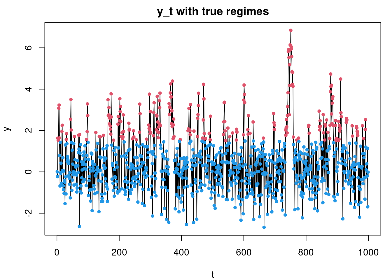
note: Equation 103.3 is a threshold autoregressive (TAR) model with two regimes.
Sample T = 1, 000 observations from model (1.1) with d = 1 using your preferred choice of values for \theta, \phi(i), and v_i for i = 1, 2, with \mid \phi(i)\mid < 1 and \phi(1) \neq \phi(2).
Assuming that d is known and using prior distributions of the form
p(\phi(i)) = \mathcal{N}(0, c)
for i = 1, 2 and some c > 0, p(\theta) = \mathcal{U}(\theta\mid −a, a)
and
p(v) = \mathcal{IG}(\alpha_0, \beta_0),
with
a > 0,
\alpha_0 > 0, and
\beta_0 > 0,
obtain samples from the joint posterior distribution by implementing a Metropolis-Hastings algorithm
TipSolution:
Simulation with:
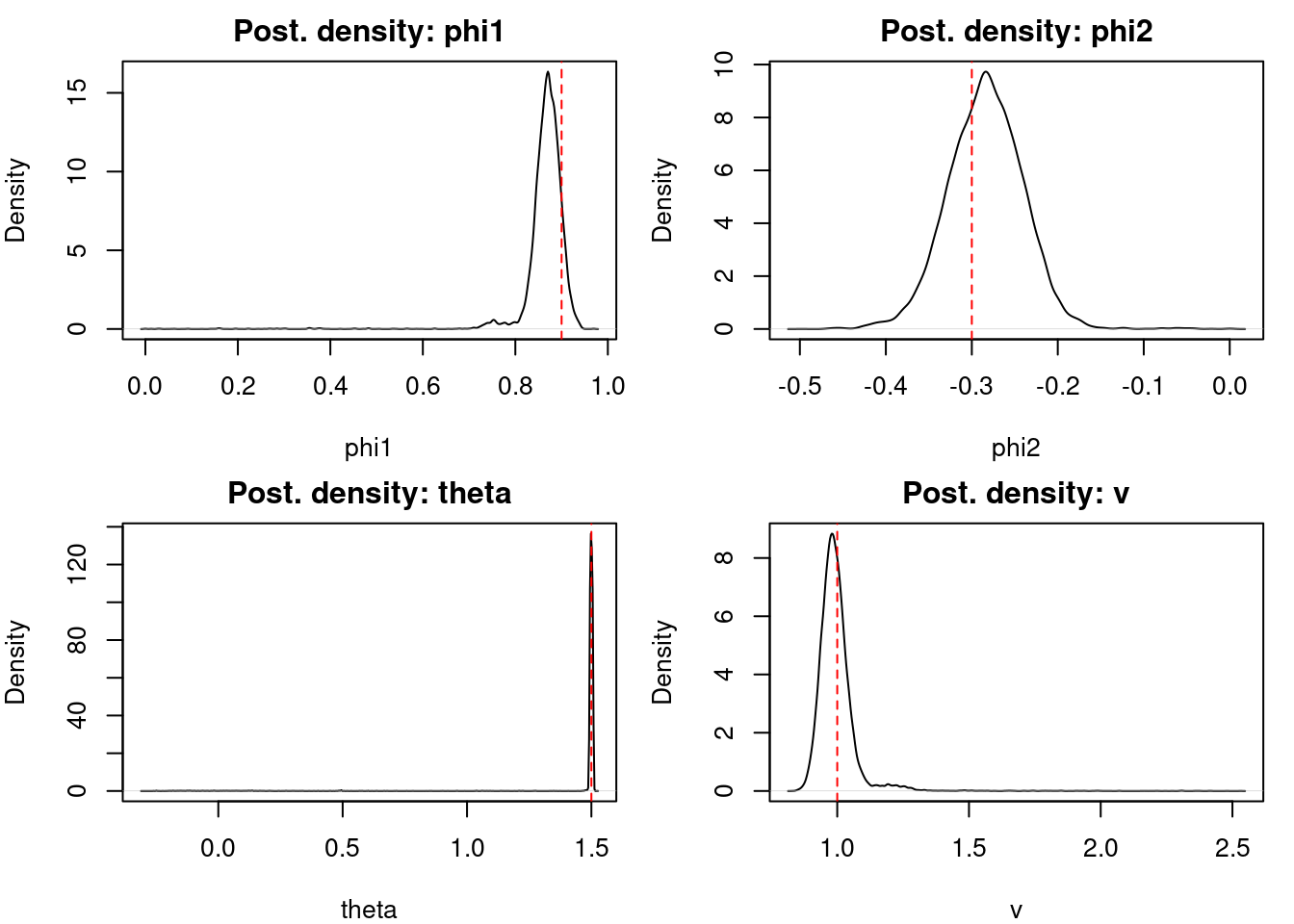
T=1000 from \phi_1=0.9, \phi_2=–0.3, \theta=1.5, \nu=1.
Uses priors:
\phi_i \sim \mathcal{N}(0, c),
\theta \sim \mathcal{U}(−a,a),
\nu \sim \mathcal{IG}(\alpha_0,\beta_0).
The regime is known corresponding to an externally triggered threshold.
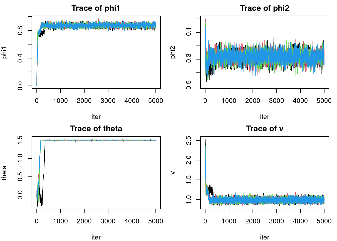
Proposes \phi_1, \phi_2, \theta by Gaussian random walk; Gibbs‐samples \nu.
We runs 4 chains, plots data+regimes, traces and posterior densities.
set.seed(123)############################## 1. simulate data #############################sim_TAR <-function(T, phi1, phi2, theta, v) { y <-numeric(T) eps <-rnorm(T, 0, sqrt(v))for(t in2:T) { y[t] <- (if(y[t-1] > theta) phi1*y[t-1] else phi2*y[t-1]) + eps[t] } y}y <-sim_TAR(1000, 0.9, -0.3, 1.5, 1)############################## 2. log‐posterior #############################log_post <-function(params, y, c, a, alpha0, beta0) { φ1 <- params[1]; φ2 <- params[2]; θ <- params[3] T <-length(y)# regime assignments r <-ifelse(y[-T] > θ, 1, 2) preds <-ifelse(r==1, φ1*y[-T], φ2*y[-T]) resid <- y[-1] - preds# sample variance posterior parameters ssq <-sum(resid^2)# log-likelihood (marginalizing v via IG: we’ll do Gibbs, so here use conditional on current v)# but for MH-we only need terms involving φ,θ up to constant ll <--0.5* ssq # since we'll compare ratios, omit log(v) term# priors lp_phi1 <--φ1^2/(2*c) lp_phi2 <--φ2^2/(2*c) lp_theta<-if(abs(θ)<=a) 0else-Inf ll + lp_phi1 + lp_phi2 + lp_theta}############################## 3. one‐chain sampler#############################run_chain <-function(y, n_iter=5000, c=10, a=5, alpha0=2, beta0=2,prop_sd =c(0.05,0.05,0.05)) {# storage chain <-matrix(NA, n_iter, 4) # φ1,φ2,θ,v# init phi1 <-0; phi2 <-0; theta <-0; v <-1for(i in1:n_iter) { curr <-c(phi1,phi2,theta) lp0 <-log_post(curr,y,c,a,alpha0,beta0) - (length(y)-1)/2*log(v) - beta0/v# MH updates for φ1, φ2, θfor(j in1:3) { prop <- curr prop[j] <-rnorm(1, curr[j], prop_sd[j]) lp1 <-log_post(prop,y,c,a,alpha0,beta0) - (length(y)-1)/2*log(v) - beta0/vif(log(runif(1)) < lp1 - lp0) { curr <- prop; lp0 <- lp1 } }# Gibbs sample v | rest resid <- y[-1] -ifelse(y[-length(y)]>curr[3], curr[1]*y[-length(y)], curr[2]*y[-length(y)]) ssq <-sum(resid^2) shape <- (length(y)-1)/2+ alpha0 rate <- ssq/2+ beta0 v <-1/rgamma(1, shape=shape, rate=rate)# record chain[i,] <-c(curr, v) phi1 <- curr[1]; phi2 <- curr[2]; theta <- curr[3] }colnames(chain) <-c("phi1","phi2","theta","v")as.data.frame(chain)}############################## 4. run 4 chains #############################chains <-lapply(1:4, function(k) run_chain(y))############################## 5. plots ############################## (a) data + true regimespar(mfrow=c(1,1), mar=c(4,4,2,1))plot(y, type="l", main="y_t with true regimes", xlab="t", ylab="y")points(which(y[-length(y)]>1.5), y[-length(y)][y[-length(y)]>1.5], col=2, pch=20)points(which(y[-length(y)]<=1.5), y[-length(y)][y[-length(y)]<=1.5], col=4, pch=20)
par(mfrow=c(2,2), mar=c(4,4,2,1))# (b) trace & posterior for each chainfor(param inc("phi1","phi2","theta","v")) {matplot(sapply(chains, "[[", param), type='l', lty=1,main=paste0("Trace of ",param), ylab=param, xlab="iter")}
Note: when the threshold is a dependent variable, the model may be called a SETAR or (Self-Exciting Threshold Autoregressive) model. TAR models are simple non linear autoregressive models that switch between different linear regimes based on the value of the previous observation.
Some examples of SETAR models are
inflation and unemployment rate in the US,
stock market volatility in bear and bull markets,
Prado, R., M. A. R. Ferreira, and M. West. 2023. Time Series: Modeling, Computation, and Inference. Chapman & Hall/CRC Texts in Statistical Science. CRC Press.
Source Code
---title: "Q&A for Chapter 1"subtitle: "Time Series: Modeling, Computation, and Inference"bibliography: references.bib---<!-- 1. Consider putting each problem into a separate file and importing them here.This will reduce caching and build time, and allow you to edit the problems without rebuilding the entire document. Also it can help with version control, as you can track changes to each problem individually.Also it can help keep document to a more manageable length as this will keep growing as new problems are added.2. Adding per problem metadata will allow create a problem set that is better suited to specific topics.-->## Chapter 1 ProblemsProblems from p.32 of the book.::: {.callout-tip}### Overthinking Memory in Time SeriesThe ACF or autocorrelation function is a measure of the correlation between a time series and its lagged values. People talk about the memory and memorylessness of distribution and autoregressive processes. But these are often intuitively understood rather than rigorously defined. It turns out that while this **mental model** of memory in time series etc is useful, it will only get us so far and eventually may become counterproductive. Unfortunately I cannot give you a definite answer of how to map the mental model to mathematical rigor. The best I can do is point out that there are a number of formal definitions that seem to map to our intuitive understanding of memory.- ACF, Autocorrelation function (ACF), - PACF, Partial autocorrelation function (PACF),- Stationarity, - Strict stationarity, - Weak stationarity,- Order of a TS process like p in AR(p) and q in MA(q),- Periodicity, and - Pseudo-periodicity a nemesis of stationarity.These are the cognates of intuitive memory that I learned in the coursera Bayesian specialization. Looking further a field, there is the Markov property, which is a formal definition of memorylessness, where we say that a process is Markovian if the future is independent of the past given the present. However when it comes to more general models like NDLMsAll this brings us to the first problem, This is an ACF derivation from assumption of stationary for $AR(1)$ model. However we are in the part of the book that is concerned with generalities and so the next problem set will delve deeper in AR(P) models and here we look at the AR(1) which is the simplest example and amenable to pen and paper analysis.::::::: {#exr-pfw-1-7-1}Show that the autocorrelation function (ACF) of an $AR(1)$ is$\rho(h) = \phi^{\mid h\mid } \qquad h = 0, \pm 1, \pm 2, \ldots$- where: 1. the process parameter $\phi$ with $|\phi| <1$, 2. with innovation $\varepsilon \sim \mathcal{N}(0, v)$ 3. and $\rho(\varepsilon_t, \varepsilon_s)=0$ i.e. uncorrelated innovations.::::::: {.solution .callout-tip collapse="true"}#### Solution:$$Y_t = \phi Y_{t-1} + \overbrace{\varepsilon_t}^{\text{innovation}}, \quad \varepsilon_t \sim \mathcal{N}(0, v), \quad |\phi| < 1$$We assume strict stationarity and zero mean $\mathbb{E}[Y_t] = 0$1. The variance of $AR(1)$ process is given by:$$\begin{aligned}\sigma^2 &= \mathrm{Var}(Y_t) & \text{by stationarity} \\&= \mathrm{Var}(\phi Y_{t-1} + \varepsilon_t) & \text{subst. AR(1)} \\&= \mathrm{Var}(\phi Y_{t-1})+\mathrm{Var}(\varepsilon_t) & Var[A+B]=Var[A]+Var[B]\\&= \mathrm{Var}(\phi Y_{t-1}) + v & \text{prop. of normal} \\&= \phi^2 \mathrm{Var}(Y_{t-1}) + v & Var[k\times X]=k^2Var[X]\\&= \phi^2 \sigma^2 + v & \text{by stationarity} \\&= \frac{v}{1 - \phi^2} & \text{rearranging} \\\end{aligned}$$2. The autocovariance function (ACF) is given by:$$\begin{aligned}\gamma(h) &= \mathbb{C}ov(Y_t, Y_{t-h}) && \text{defn. of }\gamma(h)\\ &= \mathbb{E} [(Y_t Y_{t-h}] - \mathbb{E} [Y_t] \mathbb{E} [Y_{t-h}] && \text{prop. of } \mathbb{C}ov\\ &= \mathbb{E}[Y_t Y_{t-h}] - \cancel{\mathbb{E} [Y_t] \mathbb{E} [Y_{t-h}] } && \text{independence} \\&= \mathbb{E}[Y_t Y_{t-h}]\\ &= \mathbb{E}\big[(\phi Y_{t-1}+\varepsilon_t) Y_{t-h}\big] && \text{substitute } Y_t=\phi Y_{t-1}+\varepsilon_t\\ &= \phi \mathbb{E}[Y_{t-1}Y_{t-h}] + \mathbb{E}[\varepsilon_t Y_{t-h}] && \text{linearity of expectation}\\ &= \phi \mathbb{E}[Y_{t-1}Y_{t-h}] + \underbrace{\mathbb{E}[\varepsilon_t] }_{0}\mathbb{E}[Y_{t-h}] && \text{independence, and 0 mean for} \varepsilon \\ &= \phi \gamma(h-1) && \text{for } h \ge 1\end{aligned}$$3. The autocorrelation function (ACF) is given by:$$\begin{aligned}\rho(h) &= \frac{\mathrm{Cov}(Y_t, Y_{t+h})}{\sigma^2} \\ &= \frac{\phi^{|h|} \sigma^2}{\sigma^2} \\ &= \phi^{|h|}\end{aligned}$$::::::: {#exr-pfw-1-7-2}2. Consider the $AR(1)$ model:$$y_t = \phi y_{t−1} + \varepsilon_t \quad \varepsilon_t \sim \mathcal{N}(0, v)$$ 1. Find the *MLE* of $(\phi, v)$ for the conditional likelihood. 2. Find the *MLE* of $(\phi, v)$ for the unconditional likelihood [@prado2023time § 1.17] 3. Assume that $v$ is known. Find the *MAP estimator* of $\phi$ under a uniform prior $p(\phi) = \mathcal{U}(\phi\mid −1, 1)$ for - the conditional likelihood and - the unconditional likelihoods.::::Comment: We talk about three types of point estimates in Bayesian analysis. They are:1. **Maximum Likelihood Estimation (MLE)**: This is the most common method, where we find the parameter values that maximize the likelihood function. This is actually the frequentist approach, as it does not incorporate prior beliefs about the parameters. We like to use it as it can show us what a frequentist might report as a point estimate, and we can use it as a baseline in Bayesian analysis.2. **MAP Estimation**: The Maximum A Posteriori (MAP) estimate is the mode of the posterior distribution and can be seen as a compromise between MLE and Bayesian estimation. In this case, we also need a prior and we can use a reference prior, a uniform prior or a conjugate prior.3. **Least Squares Estimation**: This is a special case of MLE where we minimize the sum of squared residuals. It is often arises when we can look at a model as a linear regression models.So although as Bayesians we are less concerned with point estimates, questions about these may come out of the blue, and we should be able to not only answer them, but also understand the differences between them and justify our choice of prior if we use MAP estimation.::: {.solution .callout-tip collapse="true"}#### Solution:1. **Conditional likelihood** The conditional log‐likelihood (conditioning on $y_1$) is $$ \ell_c(\phi,v) = -\frac{T-1}{2}\log v - \frac{1}{2v}\sum_{t=2}^T (y_t - \phi y_{t-1})^2. $$ Maximizing in $\phi$ and $v$ gives $$ \hat\phi_c = \frac{\sum_{t=2}^T y_t y_{t-1}}{\sum_{t=2}^T y_{t-1}^2}, \qquad \hat v_c = \frac{1}{T-1}\sum_{t=2}^T (y_t - \hat\phi_c y_{t-1})^2. $$2. **Unconditional (stationary) likelihood** \[@prado2023time § 1.17] Including the marginal $y_1\sim \mathcal{N}(0,v/(1-\phi^2))$, the log‐likelihood is $$ \ell_u(\phi,v) = -\frac12\log\!\bigl(v/(1-\phi^2)\bigr) -\frac{1-\phi^2}{2v}y_1^2 -\frac{T-1}{2}\log v -\frac{1}{2v}\sum_{t=2}^T (y_t - \phi y_{t-1})^2. $$ Solving $\frac{\partial\ell_u}{\partial\phi}=0$ and $\frac{\partial\ell_u}{\partial v}=0$ yields $$ \hat\phi_u = \frac{\sum_{t=2}^T y_{t-1}y_t}{\sum_{t=2}^T y_{t-1}^2 + y_1^2}, \qquad \hat v_u = \frac{1}{T}\Bigl[(1-\hat\phi_u^2) y_1^2 + \sum_{t=2}^T (y_t - \hat\phi_u y_{t-1})^2\Bigr]. $$3. **MAP with known $v$ and $\phi\sim \mathcal{U}(-1,1)$** With a flat prior on $|\phi|<1$, the posterior is proportional to the likelihood (conditional or unconditional) on that interval. Hence the MAP equals the corresponding MLE, provided it lies in $(-1,1)$; otherwise, the posterior mode is at the nearest boundary $\phi=\pm1$. Specifically: $$ \hat\phi_{\text{MAP},c} = \hat\phi_c, \qquad \hat\phi_{\text{MAP},u} = \hat\phi_u, $$ truncated to $[-1,1]$ if necessary.::::::: {#exr-pfw-1-7-3}3. Show that under the reference analysis discussed in [@prado2023time § 1.5.3] where we assume a prior $p(\beta , v) \propto 1/v$ The corresponding posterior density is $p(\beta, v\mid y, F) \propto p(y\mid F, \beta, v)/v$ 1. the marginal posterior:$$p(\beta \mid y, F) = c(n, p) \|FF^\top\|^{\frac{1}{2}} \{1 + (\beta − \hat{\beta} )^\top FF^\top (\beta − \hat{\beta} )/(n − p)s^2 \}^{−n/2}$$where $c(n,p) = \frac{\Gamma(n/2)}{[\Gamma((n − p)/2)(s^2 \pi(n − p))^{p/2}]}$,2. The marginal density:$$p(y\mid F) = \int p(y\mid F, \beta , v)p(\beta , v)d\beta dv$$ ::::Comment: I think We mentioned **reference analysis** in course two of the specialization but I assumed a base line model. This looks pretty scary at first glance. However, I recall seeing Student t's t-distribution appearing out of the blue in a couple of places, could it be due to the reference analysis i.e. introducing a Jeffreys prior? I think so!::: {.solution .callout-tip collapse="true"}#### Solution:Let $y\in\mathbb R^{n}$, $F\in\mathbb R^{p\times n}$, $\beta\in\mathbb R^{p}$,model $y\mid\beta,v \sim \mathcal N(F^\top\beta, v I_n)$, and prior $p(\beta,v)\propto 1/v$ [@prado2023time §1.5.3]---### 0. Posterior kernel$$\begin{aligned}p(\beta,v\mid y,F) &\propto p(y\mid F,\beta,v) p(\beta,v) \\&\propto v^{-n/2}\exp\!\left[-\frac{(y-F^\top\beta)^\top(y-F^\top\beta)}{2v}\right] \frac{1}{v} \\&\propto v^{-(n/2+1)}\exp\!\left[-\frac{SSE(\beta)}{2v}\right]\end{aligned}$$with $SSE(\beta)=(y-F^\top\beta)^\top(y-F^\top\beta)$. Hence the required statement $p(\beta,v\mid y,F)\propto p(y\mid F,\beta,v)/v$ is immediate.---Define$$Q = FF^\top,\qquad \hat\beta = Q^{-1}F y,\qquad SSE_0 = (y-F^\top\hat\beta)^\top(y-F^\top\hat\beta)=(n-p)s^2 .$$Use the standard quadratic decomposition$$SSE(\beta)= (\beta-\hat\beta)^\top Q (\beta-\hat\beta) + SSE_0 .$$---### 1. Marginal posterior of $\beta$Integrate out $v$:$$\begin{aligned}p(\beta\mid y,F) &\propto \int_0^\infty v^{-(n/2+1)} \exp\!\left[-\frac{(\beta-\hat\beta)^\top Q (\beta-\hat\beta) + SSE_0}{2v}\right] dv \\&\propto \left[1+\frac{(\beta-\hat\beta)^\top Q (\beta-\hat\beta)}{(n-p)s^2}\right]^{-n/2}.\end{aligned}$$Normalizing gives a multivariate $t$:$$p(\beta\mid y,F)= c(n,p) |Q|^{1/2}\left\{1+\frac{(\beta-\hat\beta)^\top Q (\beta-\hat\beta)}{(n-p)s^2}\right\}^{-n/2},$$with$$c(n,p)=\frac{\Gamma(n/2)}{\Gamma((n-p)/2) [\pi (n-p)s^2]^{p/2}}.$$as required.---### 2. Marginal likelihood (evidence)Integrate out $\beta$ first, then $v$:$$\int \exp\!\left[-\frac{(\beta-\hat\beta)^\top Q (\beta-\hat\beta)}{2v}\right] d\beta= (2\pi v)^{p/2} |Q|^{-1/2}.$$Thus$$\begin{aligned}p(y\mid F) &= \int_0^\infty \int p(y\mid F,\beta,v) p(\beta,v) d\beta dv \\&= (2\pi)^{-(n-p)/2}|Q|^{-1/2} \int_0^\infty v^{-(n-p)/2-1}\exp\!\left[-\frac{SSE_0}{2v}\right] dv \\&= |Q|^{-1/2} \frac{\Gamma\!\left(\frac{n-p}{2}\right)} {\big[\pi SSE_0\big]^{(n-p)/2}} \\&= |FF^\top|^{-1/2} \frac{\Gamma\!\left(\frac{n-p}{2}\right)} {\big[\pi (n-p) s^2\big]^{(n-p)/2}} .\end{aligned}$$::::::: {#exr-pfw-1-7-4}Show that the distributions of $(\phi\mid y, F)$ and $(v\mid y, F)$ obtained for the AR(1) reference analysis using the conditional likelihood are those givenin [@prado2023time Example 1.6], i.e. **Reference analysis in the AR(1) model.**Assume the AR(1) model :- $y = (y_2 , \ldots , y_T )^\top , F =(_y1 , \ldots , y_{T −1} )$ and - the reference prior $p(\phi, v) \propto 1/v$$(\phi\mid y, F) \sim t_{(T −2)} (m,\frac{C}{T − 2})$,where $m = \frac{ \sum_{t=2}^T y_t y_{t−1}}{\sum_{t=1}^{T-1} y^2}$ and $C = \frac{\sum_{t=2}^T y_t^2 {\sum_{t=2}^{T} y_t-1}^2 - \sum_{t=2}^T (y_t y_{t−1})^2}{\sum_{t=1}^{T-1} y_t^2}$.$(v\mid y, F) \sim \mathcal{IG}\left (\frac{T − 2}{2}, \frac{(T − 2)s^2}{2}\right)$,where $m = \frac{1}{T − 1} \sum_{t=2}^T y_t y_{t−1}$ and $SSE(\phi) = \sum_{t=2}^T (y_t − m y_{t−1})^2$. :::::::: {#exr-pfw-1-7-5}5. Show that the expressions for the distributions of $(y\mid F, v)$, $(v\mid y, F)$, and $(\beta \mid y, F)$ under the **conjugate analysis** in [@prado2023time § 1.5.3] are those given on page 24.i.e.$$(y|F, v) \sim \mathcal{N} (F^\top m_0, v(F^\top C_0 F + I_n))$$$$(v|y, F) \sim \mathcal{IG}(n^* /2, d^* /2)$$- with - $n^* = n + n_0$ and - $d^* = (y − F^\top m_0 )^\top Q^{-1} (y − F^\top m_0 ) + d_0$$$(\beta|y, F) ∼ T_{n^*} [m, d^* C/n^* ].$$::::::: {.solution .callout-tip collapse="true"}#### Solution:...::::::: {#exr-pfw-1-7-6}Show that the distributions of $(\phi \mid \mathbf{y}, \mathbf{F})$ and $(v \mid \mathbf{y}, \mathbf{F})$ obtained for the AR(1) conjugate analysis using the conditional likelihood are those givenin Example 1.7.Assume we choose a prior of the form :$\phi|v \sim \mathcal{N} (0, v)$ and$v \sim \mathcal{IG}(n0 /2, d0 /2)$, with $n0$ and $d0$ known.1. $(\phi \mid \mathbf{y}, \mathbf{F}) \sim \mathcal{N} (m, vC)$2. $(v \mid \mathbf{y}, \mathbf{F}) \sim \mathcal{IG}(n^*/2, d^*/2)$- where - $n^* = n + n_0$ and - $d^* = (y − F^\top m)^\top Q^{-1} (y − F^\top m) + d_0$.::::::: {.solution .callout-tip collapse="true"}#### Solution:...::::::: {#exr-pfw-1-7-7}Consider the following models:$$y_t= \phi_1 y_{t−1} + \phi_2 y_{t−2} + \varepsilon_t \qquad (1.26)$$ {#eq-model-1-26}$$y_t= a \cos(2\pi \omega_0 t) + b \sin(2\pi \omega_0 t) + \varepsilon_t \qquad (1.27)$$ {#eq-model-1-27}- with - $\varepsilon_t \sim \mathcal{N} (0, v)$ - and $\omega_0 > 0$ fixed. 1. Sample $T = 200$ observations from each model using your favorite choice of the parameters. Make sure your choice of $(\phi_1 , \phi_2 )$ in model (@eq-model-1-26) lies in the stationary region. That is, choose $\phi_1$ and $\phi_2$ such that $−1 < \phi_2 < 1$, $\phi_1 < 1 − \phi_2$, and $\phi_1 > \phi_2 − 1$. 2. Find the MLEs of the parameters in models (@eq-model-1-26) and (@eq-model-1-27). Use the conditional likelihood for model (@eq-model-1-26). 3. Find the MAP estimators of the model parameters under the reference prior. Again, use the conditional likelihood for model (@eq-model-1-26). 4. Sketch $p(v\mid y, F)$ and $p(\phi_1 , \phi_2 \mid y, F)$ for model (@eq-model-1-26). 5. Sketch $p(a, b\mid y, F)$ and $p(v\mid y, F)$ for model (@eq-model-1-27). 6. Perform a conjugate Bayesian analysis, i.e., repeat 3-4 assuming conjugate prior distributions in both models. Study the sensitivity of the posterior distributions to the choice of the hyperparameters in the prior.::::::: {.solution .callout-tip collapse="true"}#### Solution:```{python}#| label: lst-pfw-1-7-7# Exercise 1.7-7: AR(2) and Sinusoidal Models########################################################### This script solves the six tasks in Exercise 1.7-7:# 1. Simulate T=200 observations from an AR(2) model and a sinusoidal model.# 2. Compute MLEs of parameters using conditional likelihood for AR(2) and OLS for sinusoid.# 3. Compute MAP estimators under the reference prior p(φ,v) ∝ 1/v.# 4. Sketch posterior p(v|y,F) and p(φ₁,φ₂|y,F) for AR(2).# 5. Sketch posterior p(a,b|y,F) and p(v|y,F) for the sinusoidal model.# 6. Perform conjugate Bayesian analysis for both models and study sensitivity.import numpy as npimport matplotlib.pyplot as pltfrom scipy.stats import invgamma############################## Part 1: Simulation#############################def simulate_ar2(phi, sigma2, T, seed=None):""" Generate AR(2) data: y_t = φ₁ y_{t−1} + φ₂ y_{t−2} + ε_t, ε_t∼N(0,σ²). Returns array of length T. """if seed isnotNone: np.random.seed(seed) y = np.zeros(T) eps = np.random.normal(0, np.sqrt(sigma2), size=T)for t inrange(2, T): y[t] = phi[0]*y[t-1] + phi[1]*y[t-2] + eps[t]return ydef simulate_sin(ab, omega0, sigma2, T, seed=None):""" Generate sinusoidal data: y_t = a cos(2π ω₀ t) + b sin(2π ω₀ t) + ε_t. Returns time index and observations. """if seed isnotNone: np.random.seed(seed) t = np.arange(1, T+1) a, b = ab deterministic = a*np.cos(2*np.pi*omega0*t) + b*np.sin(2*np.pi*omega0*t) noise = np.random.normal(0, np.sqrt(sigma2), size=T)return t, deterministic + noise############################## Part 2: Maximum Likelihood#############################def mle_ar2(y):""" MLE for AR(2) via OLS on y[2:] ~ y[1:-1], y[:-2]. Returns φ̂ = [φ₁,φ₂], σ̂². """ Y = y[2:] X = np.column_stack([y[1:-1], y[:-2]]) phi_hat, *_ = np.linalg.lstsq(X, Y, rcond=None) resid = Y - X.dot(phi_hat) sigma2_hat = np.mean(resid**2)return phi_hat, sigma2_hatdef mle_sin(y, omega0):""" MLE for sinusoid via OLS on y ~ cos(2πω₀t), sin(2πω₀t). Returns [â,b̂], σ̂². """ T =len(y) t = np.arange(1, T+1) X = np.column_stack([ np.cos(2*np.pi*omega0*t), np.sin(2*np.pi*omega0*t) ]) ab_hat, *_ = np.linalg.lstsq(X, y, rcond=None) resid = y - X.dot(ab_hat) sigma2_hat = np.mean(resid**2)return ab_hat, sigma2_hat############################## Part 3: MAP under Reference Prior#############################def map_ref_ar2(y):""" MAP under p(φ,v) ∝ 1/v for AR(2). φ̂ same as MLE, v̂ = (SSE/2)/(n/2 + 1). """ Y = y[2:]; X = np.column_stack([y[1:-1], y[:-2]]) phi_mle, sigma2_mle = mle_ar2(y) resid = Y - X.dot(phi_mle) n =len(Y) SSE = resid.dot(resid) alpha, beta = n/2, SSE/2 v_map = beta/(alpha +1)return phi_mle, v_mapdef map_ref_sin(y, omega0):""" MAP under p(a,b,v) ∝ 1/v for sinusoid. (a,b)̂ same as MLE, v̂ MAP as above. """ ab_hat, _ = mle_sin(y, omega0) t = np.arange(1, len(y)+1) X = np.column_stack([ np.cos(2*np.pi*omega0*t), np.sin(2*np.pi*omega0*t) ]) resid = y - X.dot(ab_hat) n =len(y) SSE = resid.dot(resid) alpha, beta = n/2, SSE/2 v_map = beta/(alpha +1)return ab_hat, v_map############################## Part 4 & 5: Posterior Sketches#############################def plot_posteriors_ar2(phi_map, y):""" Plot posterior contours for φ and density for v under reference prior. """ Y = y[2:]; X = np.column_stack([y[1:-1], y[:-2]]) phi_hat = phi_map A_inv = np.linalg.inv(X.T.dot(X))# φ posterior: approx N(phi_hat, v*inv(X'X)) scaled out v grid = np.linspace(-1,1,80) P1,P2 = np.meshgrid(grid+phi_hat[0], grid+phi_hat[1]) invA = np.linalg.inv(A_inv) norm =1/(2*np.pi*np.sqrt(np.linalg.det(A_inv))) Z = norm * np.exp(-0.5*( invA[0,0]*(P1-phi_hat[0])**2+2*invA[0,1]*(P1-phi_hat[0])*(P2-phi_hat[1]) + invA[1,1]*(P2-phi_hat[1])**2 )) plt.contour(P1,P2,Z) plt.title("p(φ₁,φ₂|y)"); plt.xlabel('φ₁'); plt.ylabel('φ₂') plt.show() resid = Y - X.dot(phi_hat) n =len(Y); SSE = resid.dot(resid) alpha,beta = n/2, SSE/2 v_grid = np.linspace(0.01, np.max(resid**2), 200) plt.plot(v_grid, invgamma.pdf(v_grid, a=alpha, scale=beta)) plt.title("p(v|y)"); plt.xlabel('v'); plt.show()def plot_posteriors_sin(ab_map, omega0, y):""" Plot posterior contours for (a,b) and density for v under reference prior. """ a_hat,b_hat = ab_map t = np.arange(1, len(y)+1) X = np.column_stack([ np.cos(2*np.pi*omega0*t), np.sin(2*np.pi*omega0*t) ])# (a,b) posterior B_inv = np.linalg.inv(X.T.dot(X)) grid = np.linspace(-1,1,80) Agrid,Bgrid = np.meshgrid(grid+a_hat, grid+b_hat) invB = np.linalg.inv(B_inv) norm =1/(2*np.pi*np.sqrt(np.linalg.det(B_inv))) Z = norm * np.exp(-0.5*( invB[0,0]*(Agrid-a_hat)**2+2*invB[0,1]*(Agrid-a_hat)*(Bgrid-b_hat) + invB[1,1]*(Bgrid-b_hat)**2 )) plt.contour(Agrid,Bgrid,Z) plt.title("p(a,b|y)"); plt.xlabel('a'); plt.ylabel('b'); plt.show() resid = y - X.dot(ab_map) n =len(y); SSE = resid.dot(resid) alpha,beta = n/2, SSE/2 v_grid = np.linspace(0.01, np.max(resid**2), 200) plt.plot(v_grid, invgamma.pdf(v_grid, a=alpha, scale=beta)) plt.title("p(v|y)"); plt.xlabel('v'); plt.show()############################## Part 6: Conjugate Bayesian Analysis & Sensitivity#############################def post_conj_norminv(y, X, m0, C0, n0, d0):""" Conjugate posterior for regression y ~ Xβ + ε, ε∼N(0,v): β|v ~ N(m_n, C_n v), v∼Inv-Gamma(n_n,d_n). Returns m_n, C_n, n_n, d_n. """ C0_inv = np.linalg.inv(C0) Vn_inv = X.T.dot(X) + C0_inv Vn = np.linalg.inv(Vn_inv) mn = Vn.dot(X.T.dot(y) + C0_inv.dot(m0)) resid = y - X.dot(mn) n_n = n0 +len(y)/2 d_n = d0 +0.5*(resid.dot(resid) + (mn-m0).T.dot(C0_inv).dot(mn-m0))return mn, Vn, n_n, d_n############################## Main execution#############################T =200# True parameters in stationary regionphi_true = np.array([0.5, 0.2])sigma2 =1.0y_ar2 = simulate_ar2(phi_true, sigma2, T, seed=42)ab_true = np.array([2.0, 1.0])omega0 =0.1t_sin, y_sin = simulate_sin(ab_true, omega0, sigma2, T, seed=42)# MLEsphi_mle, s2_mle_ar2 = mle_ar2(y_ar2)ab_mle, s2_mle_sin = mle_sin(y_sin, omega0)# MAP under reference priorphi_map, s2_map_ar2 = map_ref_ar2(y_ar2)ab_map, s2_map_sin = map_ref_sin(y_sin, omega0)# Plot reference-posteriorsplot_posteriors_ar2(phi_map, y_ar2)plot_posteriors_sin(ab_map, omega0, y_sin)# Conjugate sensitivitypriors = [ (np.zeros(2), np.eye(2)*1, 1.0, 1.0), (np.zeros(2), np.eye(2)*10, 0.1, 0.1)]print("Conjugate AR(2) sensitivity:")for m0,C0,n0,d0 in priors: Y = y_ar2[2:]; X = np.column_stack([y_ar2[1:-1], y_ar2[:-2]]) mn, Vn, nn, dn = post_conj_norminv(Y, X, m0, C0, n0, d0)print(" m0={}, C0 scale={}, E[φ]={}".format(m0, np.diag(C0), mn))print("Conjugate Sinusoid sensitivity:")for m0,C0,n0,d0 in priors: Y = y_sin; X = np.column_stack([ np.cos(2*np.pi*omega0*t_sin), np.sin(2*np.pi*omega0*t_sin) ]) mn, Vn, nn, dn = post_conj_norminv(Y, X, m0[:2], C0, n0, d0)print(" m0={}, C0 scale={}, E[(a,b)]={}".format(m0[:2], np.diag(C0), mn))```::::::: {#exr-pfw-1-7-8}Refer to the conjugate analysis of the AR(1) model in Example 1.7. Using the fact that $(\phi\mid y, F, v) \sim \mathcal{N}(m, vC)$, find the posterior mode of $v$ via the EM algorithm.::::::: {.solution .callout-tip collapse="true"}#### Solution:```{python}#| label: lst-pfw-1-7-8import numpy as npimport matplotlib.pyplot as pltfrom scipy.stats import invgamma############################## 1. Simulation#############################def simulate_ar2(phi, sigma, T, seed=0): np.random.seed(seed) y = np.zeros(T) eps = np.random.normal(0, sigma, size=T)for t inrange(2, T): y[t] = phi[0]*y[t-1] + phi[1]*y[t-2] + eps[t]return ydef simulate_sin(ab, omega0, sigma, T, seed=0): np.random.seed(seed) t = np.arange(1, T+1) a, b = ab signal = a*np.cos(2*np.pi*omega0*t) + b*np.sin(2*np.pi*omega0*t)return t, signal + np.random.normal(0, sigma, size=T)############################## 2. MLE#############################def mle_ar2(y): Y = y[2:]; X = np.column_stack([y[1:-1], y[:-2]]) phi_hat = np.linalg.lstsq(X, Y, rcond=None)[0] resid = Y - X.dot(phi_hat) v_hat = np.mean(resid**2)return phi_hat, v_hatdef mle_sin(y, omega0): T =len(y) t = np.arange(1, T+1) X = np.column_stack([np.cos(2*np.pi*omega0*t), np.sin(2*np.pi*omega0*t)]) ab_hat = np.linalg.lstsq(X, y, rcond=None)[0] resid = y - X.dot(ab_hat) v_hat = np.mean(resid**2)return ab_hat, v_hat############################## 3. Reference-prior posterior (MAP)#############################def map_ref_ar2(y): Y = y[2:]; X = np.column_stack([y[1:-1], y[:-2]]) phi_hat = np.linalg.lstsq(X, Y, rcond=None)[0] resid = Y - X.dot(phi_hat) n =len(Y); SSE = resid.dot(resid)# inv-Gamma post: α=n/2, β=SSE/2 --> MAP at β/(α+1) alpha, beta = n/2, SSE/2 v_map = beta/(alpha+1)return phi_hat, v_mapdef map_ref_sin(y, omega0): T =len(y) t = np.arange(1, T+1) X = np.column_stack([np.cos(2*np.pi*omega0*t), np.sin(2*np.pi*omega0*t)]) ab_hat = np.linalg.lstsq(X, y, rcond=None)[0] resid = y - X.dot(ab_hat) n =len(y); SSE = resid.dot(resid) alpha, beta = n/2, SSE/2 v_map = beta/(alpha+1)return ab_hat, v_map############################## 4. Conjugate updates#############################def post_conj_ar2(y, m0, C0, n0, d0): Y = y[2:]; X = np.column_stack([y[1:-1], y[:-2]]) C0_inv = np.linalg.inv(C0) Vn_inv = X.T.dot(X) + C0_inv Vn = np.linalg.inv(Vn_inv) mn = Vn.dot(X.T.dot(Y) + C0_inv.dot(m0)) resid = Y - X.dot(mn) n =len(Y) nn = n0 + n/2 dd = d0 +0.5*(resid.dot(resid) + (mn-m0).T.dot(C0_inv).dot(mn-m0)) v_mean = dd/(nn-1)return mn, Vn, v_meandef post_conj_sin(y, omega0, m0, C0, n0, d0): T =len(y); t = np.arange(1, T+1) X = np.column_stack([np.cos(2*np.pi*omega0*t), np.sin(2*np.pi*omega0*t)]) C0_inv = np.linalg.inv(C0) Vn_inv = X.T.dot(X) + C0_inv Vn = np.linalg.inv(Vn_inv) mn = Vn.dot(X.T.dot(y) + C0_inv.dot(m0)) resid = y - X.dot(mn) nn = n0 + T/2 dd = d0 +0.5*(resid.dot(resid) + (mn-m0).T.dot(C0_inv).dot(mn-m0)) v_mean = dd/(nn-1)return mn, Vn, v_mean############################## Main Execution#############################T =200phi_true = np.array([0.5,0.2]); sigma =1.0y_ar2 = simulate_ar2(phi_true, sigma, T)ab_true, omega0 = np.array([2.0,1.0]), 0.1t_sin, y_sin = simulate_sin(ab_true, omega0, sigma, T)# MLEphi_mle, v_mle = mle_ar2(y_ar2)ab_mle, v_sin_mle = mle_sin(y_sin, omega0)# MAP refphi_map, v_map_ar2 = map_ref_ar2(y_ar2)ab_map, v_map_sin = map_ref_sin(y_sin, omega0)# Conjugate (two priors for sensitivity)priors = [ (np.zeros(2), np.eye(2)*1, 1.0, 1.0), (np.zeros(2), np.eye(2)*10, 0.1, 0.1)]print("=== AR(2) Estimates ===")print("True φ:", phi_true, " σ²=", sigma**2)print("MLE φ,σ²:", phi_mle, v_mle)print("MAP-ref φ,σ²:", phi_map, v_map_ar2)for i,(m0,C0,n0,d0) inenumerate(priors,1): mn, Vn, v_mean = post_conj_ar2(y_ar2,m0,C0,n0,d0)print(f"Conjugate#{i} posterior mean φ:", mn, " E[σ²]:", v_mean)print("\n=== Sinusoid Estimates ===")print("True (a,b):", ab_true, " σ²=", sigma**2)print("MLE (a,b),σ²:", ab_mle, v_sin_mle)print("MAP-ref (a,b),σ²:", ab_map, v_map_sin)for i,(m0,C0,n0,d0) inenumerate(priors,1): mn, Vn, v_mean = post_conj_sin(y_sin,omega0,m0,C0,n0,d0)print(f"Conjugate#{i} posterior mean (a,b):", mn, " E[σ²]:", v_mean)```::::::: {#exr-pfw-1-7-9}Model (1.1): a time series generated from the process $$y_t =\begin{cases} 0.9y_{t−1} + \varepsilon_t^{(1)} & y_{t−1} > 1.5\ (\mathcal{M}1 ) \\ −0.3y_{t−1} + \varepsilon_t^{(2)} & y_{t−1} ≤ 1.5\ (\mathcal{M}2 ),\end{cases}$$ {#eq-model-1-1} - where - $\varepsilon_t^{(1)} \sim \mathcal{N} (0, v_1 )$, - $\varepsilon_t^{(2)} \sim \mathcal{N} (0, v_2 )$, and - $v_1 = v_2 = 1$note: @eq-model-1-1 is a **threshold autoregressive (TAR) model** with two regimes.Sample $T = 1,000$ observations from model (1.1) with $d = 1$ using your preferred choice of values for $\theta$, $\phi(i)$, and $v_i$ for $i = 1, 2$, with $\mid \phi(i)\mid < 1$ and $\phi(1) \neq \phi(2)$. Assuming that $d$ is known and using prior distributions of the form $p(\phi(i)) = \mathcal{N}(0, c)$for $i = 1, 2$ and some $c > 0$, $p(\theta) = \mathcal{U}(\theta\mid −a, a)$ and $p(v) = \mathcal{IG}(\alpha_0, \beta_0)$, - with - $a > 0$, - $\alpha_0 > 0$, and - $\beta_0 > 0$,obtain samples from the joint posterior distribution by implementing a Metropolis-Hastings algorithm::::::: {.solution .callout-tip collapse="true"}#### Solution:Simulation with:- $T=1000$ from $\phi_1=0.9, \phi_2=–0.3, \theta=1.5, \nu=1$.Uses priors:- $\phi_i \sim \mathcal{N}(0, c)$,- $\theta \sim \mathcal{U}(−a,a)$,- $\nu \sim \mathcal{IG}(\alpha_0,\beta_0)$.The regime is known corresponding to an externally triggered threshold.Proposes $\phi_1$, $\phi_2$, $\theta$ by Gaussian random walk; Gibbs‐samples $\nu$.We runs 4 chains, plots data+regimes, traces and posterior densities.```{r}#| label: lst-pfw-1-7-9set.seed(123)############################## 1. simulate data #############################sim_TAR <-function(T, phi1, phi2, theta, v) { y <-numeric(T) eps <-rnorm(T, 0, sqrt(v))for(t in2:T) { y[t] <- (if(y[t-1] > theta) phi1*y[t-1] else phi2*y[t-1]) + eps[t] } y}y <-sim_TAR(1000, 0.9, -0.3, 1.5, 1)############################## 2. log‐posterior #############################log_post <-function(params, y, c, a, alpha0, beta0) { φ1 <- params[1]; φ2 <- params[2]; θ <- params[3] T <-length(y)# regime assignments r <-ifelse(y[-T] > θ, 1, 2) preds <-ifelse(r==1, φ1*y[-T], φ2*y[-T]) resid <- y[-1] - preds# sample variance posterior parameters ssq <-sum(resid^2)# log-likelihood (marginalizing v via IG: we’ll do Gibbs, so here use conditional on current v)# but for MH-we only need terms involving φ,θ up to constant ll <--0.5* ssq # since we'll compare ratios, omit log(v) term# priors lp_phi1 <--φ1^2/(2*c) lp_phi2 <--φ2^2/(2*c) lp_theta<-if(abs(θ)<=a) 0else-Inf ll + lp_phi1 + lp_phi2 + lp_theta}############################## 3. one‐chain sampler#############################run_chain <-function(y, n_iter=5000, c=10, a=5, alpha0=2, beta0=2,prop_sd =c(0.05,0.05,0.05)) {# storage chain <-matrix(NA, n_iter, 4) # φ1,φ2,θ,v# init phi1 <-0; phi2 <-0; theta <-0; v <-1for(i in1:n_iter) { curr <-c(phi1,phi2,theta) lp0 <-log_post(curr,y,c,a,alpha0,beta0) - (length(y)-1)/2*log(v) - beta0/v# MH updates for φ1, φ2, θfor(j in1:3) { prop <- curr prop[j] <-rnorm(1, curr[j], prop_sd[j]) lp1 <-log_post(prop,y,c,a,alpha0,beta0) - (length(y)-1)/2*log(v) - beta0/vif(log(runif(1)) < lp1 - lp0) { curr <- prop; lp0 <- lp1 } }# Gibbs sample v | rest resid <- y[-1] -ifelse(y[-length(y)]>curr[3], curr[1]*y[-length(y)], curr[2]*y[-length(y)]) ssq <-sum(resid^2) shape <- (length(y)-1)/2+ alpha0 rate <- ssq/2+ beta0 v <-1/rgamma(1, shape=shape, rate=rate)# record chain[i,] <-c(curr, v) phi1 <- curr[1]; phi2 <- curr[2]; theta <- curr[3] }colnames(chain) <-c("phi1","phi2","theta","v")as.data.frame(chain)}############################## 4. run 4 chains #############################chains <-lapply(1:4, function(k) run_chain(y))############################## 5. plots ############################## (a) data + true regimespar(mfrow=c(1,1), mar=c(4,4,2,1))plot(y, type="l", main="y_t with true regimes", xlab="t", ylab="y")points(which(y[-length(y)]>1.5), y[-length(y)][y[-length(y)]>1.5], col=2, pch=20)points(which(y[-length(y)]<=1.5), y[-length(y)][y[-length(y)]<=1.5], col=4, pch=20)par(mfrow=c(2,2), mar=c(4,4,2,1))# (b) trace & posterior for each chainfor(param inc("phi1","phi2","theta","v")) {matplot(sapply(chains, "[[", param), type='l', lty=1,main=paste0("Trace of ",param), ylab=param, xlab="iter")}# (c) marginal posterior densitiespar(mfrow=c(2,2))for(param inc("phi1","phi2","theta","v")) { dens <-density(unlist(lapply(chains, "[[", param)))plot(dens, main=paste0("Post. density: ",param), xlab=param)abline(v =if(param=="phi1") 0.9elseif(param=="phi2") -0.3elseif(param=="theta") 1.5else1, col="red", lty=2)}```:::Note: when the threshold is a dependent variable, the model may be called a SETAR or (Self-Exciting Threshold Autoregressive) model. TAR models are simple non linear autoregressive models that switch between different linear regimes based on the value of the previous observation.Some examples of SETAR models are- inflation and unemployment rate in the US,- stock market volatility in bear and bull markets,