In this lesson we will present and then prove Dynkin’s \pi-\lambda theorem, which gives a powerful criterion for showing that a \lambda-system contains the \sigma-field generated by a \pi-system. We then apply this result to show that independent \pi-systems generate independent \sigma-fields.
155.1 Lesson map
- Recap: independence of events and independence of classes of events
- Definition of independent classes using \Omega to encode lower-order intersections.
- Counterexample: independent classes need not generate independent \sigma-fields.
- Definition of a \pi-system.
- Definition of a \lambda-system.
- Equivalent proper-difference condition for \lambda-systems.
- A class that is both a \pi-system and a \lambda-system is a \sigma-field.
- Intersections of \lambda-systems.
- The auxiliary class \mathcal{L}_A=\{B:A\cap B\in\mathcal{L}\}.
- Dynkin’s \pi-\lambda theorem.
- Independent \pi-systems generate independent \sigma-fields.
- Extension to infinite families by checking finite subfamilies.
155.2 Recap: independence for classes of events
Definition 155.1 (Independence for classes of events) Let (\Omega,\mathcal{F},P), be a probability space, with collections (classes) of sets (events) \mathcal{A}_1,\mathcal{A}_2,\ldots,\mathcal{A}_n \subseteq \mathcal{F}
The classes are independent if any choice of events A_i\in\mathcal{A}_i gives independent events A_1,A_2,\ldots,A_n.
For a pair of events, independence means P(A\cap B)=P(A)P(B). For a finite family of classes, the clean version of the definition is:
Definition 155.2 (Alternative definition of independence for classes of events) Let (\Omega,\mathcal{F},P), be a probability space, with collections (classes) of sets (events) from \mathcal{A}_1,\mathcal{A}_2,\ldots,\mathcal{A}_n \subseteq \mathcal{F} are independent if
P(A_1\cap A_2\cap\cdots\cap A_n) = \prod_{i=1}^n P(A_i), \forall A_i \in \mathcal{A}_i. \text{ or } A_i=\Omega.
where each A_i is either chosen from \mathcal{A}_i or is allowed to be \Omega.
Allowing A_i=\Omega folds all lower-order intersections into the same n-fold formula.
For example, with three classes, the pairwise condition for A_1 and A_3 appears by setting A_2=\Omega:
P(A_1\cap \Omega\cap A_3) = P(A_1)P(\Omega)P(A_3) = P(A_1)P(A_3).
155.3 Todays motivating question: Does independence survive generating \sigma-fields?
Our main question today is does independence survive the operation of generating \sigma-fields:
\mathcal{A}_1,\mathcal{A}_2 \text{ independent} \quad \stackrel{???}{\Longrightarrow}\quad \sigma(\mathcal{A}_1),\sigma(\mathcal{A}_2) \text{ independent}.
Hint: The answer is not in general.
It becomes true after adding the key structural assumption: each starting class should be a \pi-system.
155.4 Why the naive theorem fails
Keeping track of the different levels of structure: events, classes of events, and \sigma-fields is confusing.
The main point jem reiterates is that the sigma-field generation operates on the classes, not on the events!
The key is to remember that a \sigma-field is a special kind of class of events, so we can talk about independence for classes and then ask if it survives when we generate \sigma-fields from those classes.
Since the notation isn’t stellar the example Example 155.1 helps to sort the three out
Example 155.1 (Counterexample: independent coin flips classes yield dependent \sigma-fields) The space for two fair coin coins: \Omega=\{HH,HT,TH,TT\},\quad \mathbb{P}(\{\omega\})=\frac14. Let define events A=\{HH,HT\}, B=\{HH,TT\}, C=\{HT,TT\} and classes \mathcal{A}_1=\{A,B\}, \quad \mathcal{A}_2=\{C\}
The classes \mathcal{A}_1 and \mathcal{A}_2 are independent. e.g. A\cap C = \{HT\}, so P(A\cap C)=\frac14 = \frac12\cdot\frac12 =P(A)P(C).
The original classes pass the independence check.
Note that C = (A\cup B)\setminus(A\cap B) = (A\cup B)\cap (A\cap B)^c \implies C \in \sigma(\mathcal{A}_1). Also C\in\mathcal{A}_2 \implies C\in\sigma(\mathcal{A}_2). The generated \sigma-fields overlap too much: they both contain C.
C isn’t independent of itself! as \mathbb{P}(C\cap C)=\mathbb{P}(C)\neq\mathbb{P}(C)^2.
\sigma(\mathcal{A}_1) \text{ and } \sigma(\mathcal{A}_2) are not independent. \blacksquare
The counterexample works because generating a \sigma-field can create a shared nontrivial event.
155.5 \pi-systems and \lambda-systems
Definition 155.3 (\pi-system) Is a class of sets closed under finite intersections:
A,B\in\mathcal{P} \quad \Longrightarrow \quad A\cap B\in\mathcal{P}.
Every field and every \sigma-field is a \pi-system. However a \pi-system
- need not contain \Omega,
- need not be closed under complements, and
- need not be closed under unions.
This is exactly why it is a weak but useful hypothesis. Billingsley introduces \pi-systems in the uniqueness part of the extension theorem (Billingsley 2012, 43).
A \pi-system remembers only intersection structure.
155.6 Defining \lambda-systems
Definition 155.4 (\lambda-system) is a class \mathcal{L} of subsets of \Omega satisfying:
- \Omega\in\mathcal{L}
- if A\in\mathcal{L}, then A^c\in\mathcal{L}
- if A_1,A_2,\ldots \in \mathcal{L} are pairwise disjoint, then \bigcup_{n=1}^{\infty}A_n\in\mathcal{L}
A \sigma-field is a \lambda-system, but a \lambda-system is weaker because countable unions are required only for disjoint sequences (Billingsley 2012, 43).
155.6.1 Alternative difference axiom for \lambda-systems
Definition 155.5 (\lambda-system) is a class \mathcal{L} of subsets of \Omega satisfying:
- \Omega\in\mathcal{L}
- if A,B\in\mathcal{L},\ A\subseteq B \quad\Longrightarrow\quad B\setminus A\in\mathcal{L}.
- if A_1,A_2,\ldots \in \mathcal{L} are pairwise disjoint, then \bigcup_{n=1}^{\infty}A_n\in\mathcal{L}
Theorem 155.1 (equivalence of \lambda-system definitions) The two definitions of \lambda-systems Definition 155.4 and Definition 155.5 are equivalent.
The second axioms in the definitions are equivalent by themselves. However they are equivalent in the presence of the other \lambda-system axioms.
Proof.
- Definition 155.5 (1.) and (2.) \Longrightarrow Definition 155.4 (2.) since we can take B=\Omega in the proper-difference condition to get A^c\in\mathcal{L}.
- Definition 155.4 (2.) and (3.) \Longrightarrow Definition 155.5 (2.) because if A\subseteq B, then A is disjoint from B\setminus A, so B\setminus A\in\mathcal{L} by the \lambda-system property.
Conversely, suppose \mathcal{L} is closed under complements and disjoint countable unions. If A,B\in\mathcal{L} and A\subseteq B, then B^c\in\mathcal{L} and A is disjoint from B^c. Therefore A\cup B^c\in\mathcal{L}.
Taking complements, (A\cup B^c)^c = A^c\cap B = B\setminus A \in\mathcal{L}.
Proper differences are often the more convenient closure rule. e.g. using proper differences to avoid reproving complement closure in every auxiliary \lambda-system.
155.6.2 A class that is both a \pi-system and a \lambda-system is a \sigma-field
Theorem 155.2 (A class that is both a \pi-system and a \lambda-system is a \sigma-field) If \mathcal{A} is both a \pi-system and a \lambda-system. Then \mathcal{A} is a \sigma-field c.f. (Billingsley 2012, 43).
The \pi-system supplies the finite intersections; the \lambda-system supplies the disjoint countable union.
Proof. The first two \sigma-field properties are immediate:
\Omega\in\mathcal{A} because \mathcal{A} is a \lambda-system, and
A\in\mathcal{A} \quad\Longrightarrow\quad A^c\in\mathcal{A} again by the \lambda-system property.
We will be disjointizing a countable union to prove \sigma-field closure.
Now take any sequence A_1,A_2,\ldots\in\mathcal{A}. These sets need not be disjoint, so define disjoint pieces:
B_1=A_1 \quad B_2=A_2\cap A_1^c \quad B_3=A_3\cap A_2^c\cap A_1^c,
and in general B_k = A_k\cap\bigcap_{j<k}A_j^c.
The complements A_j^c are in \mathcal{A} because \mathcal{A} is a \lambda-system. The finite intersections are in \mathcal{A} because \mathcal{A} is a \pi-system. Thus each B_k\in\mathcal{A}. The B_k are disjoint, so the \lambda-system property gives \bigcup_{k=1}^{\infty}B_k\in\mathcal{A}.
But \bigcup_{k=1}^{\infty}B_k = \bigcup_{k=1}^{\infty}A_k.
Therefore \mathcal{A} is closed under countable unions, and hence is a \sigma-field.
Turn arbitrary countable unions into disjoint unions by peeling off the earlier sets.
155.7 Two auxiliary \lambda-system lemmas
155.7.1 Intersections of \lambda-systems
Theorem 155.3 (Intersections of \lambda-systems) If \mathcal{L}_1 and \mathcal{L}_2 are \lambda-systems on the same underlying set \Omega, then \mathcal{L}_1\cap\mathcal{L}_2 is also a \lambda-system.
Here the intersection is an intersection of classes of sets. A set belongs to \mathcal{L}_1\cap\mathcal{L}_2 when the entire set belongs to both classes. We are not taking a set from \mathcal{L}_1 and intersecting it with a set from \mathcal{L}_2.
Proof. The proof mirrors the analogous fact for \sigma-fields:
- \Omega lies in both \mathcal{L}_1 and \mathcal{L}_2.
- If A lies in both, then A^c lies in both.
- If A_1,A_2,\ldots are disjoint and each lies in both, then \bigcup_n A_n lies in both.
155.7.2 The smallest \lambda-system containing a class
This also justifies defining the smallest \lambda-system containing a class as the intersection of all \lambda-systems containing it, exactly as generated \sigma-fields are defined by intersections of \sigma-fields (Billingsley 2012, 21).
Intersections let us speak of the smallest \lambda-system containing a given class.
Theorem 155.4 (The section lemma: \mathcal{L}_A) Let \mathcal{L} be a \lambda-system and fix A\subseteq\Omega. Define \mathcal{L}_A = \{B\subseteq\Omega: A\cap B\in\mathcal{L}\}
If A\in\mathcal{L}, then \mathcal{L}_A is a \lambda-system.
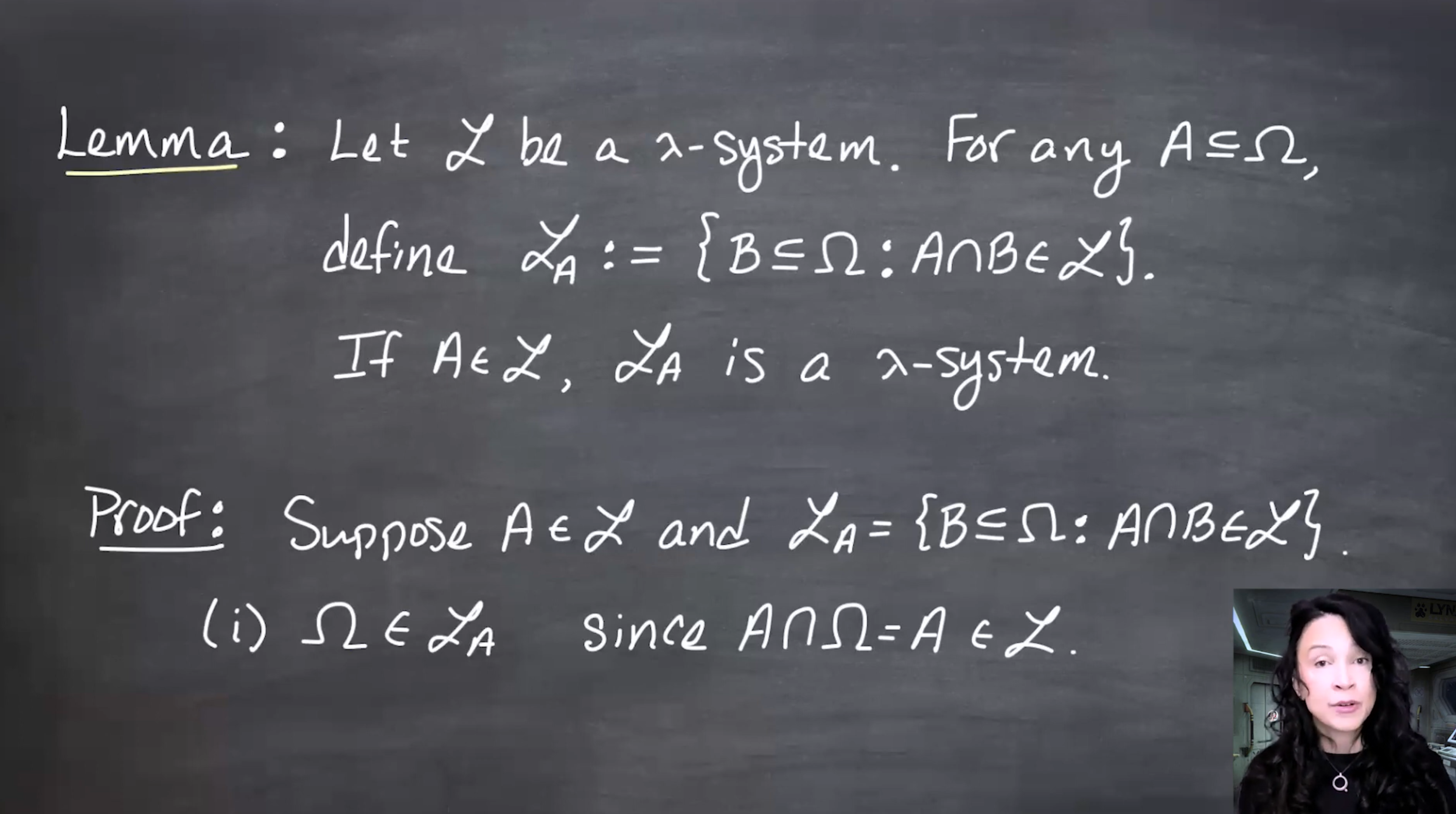
Proof. First, A\cap\Omega=A\in\mathcal{L}, so \Omega\in\mathcal{L}_A.
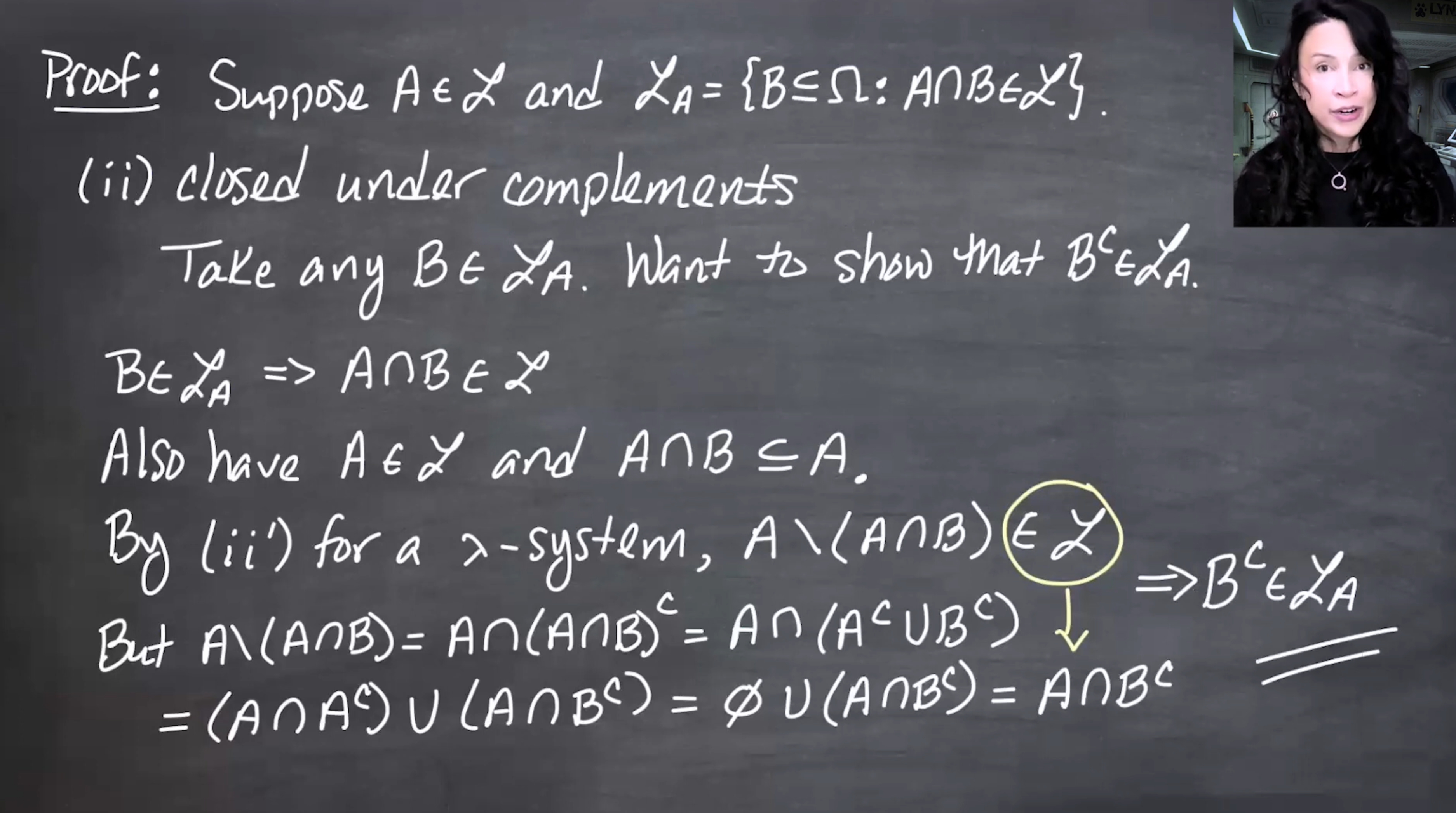
For complements, suppose B\in\mathcal{L}_A. Then
A\cap B\in\mathcal{L}, \qquad A\cap B\subseteq A, \qquad A\in\mathcal{L}.
By the proper-difference version of the \lambda-system axiom,
\begin{aligned} \mathcal{L} &\ni A\setminus(A\cap B) \\ &= A\cap(A\cap B)^c \\ &= A\cap(A^c\cup B^c) \\ &= A\cap B^c \\ &\implies B^c\in\mathcal{L}_A \end{aligned}
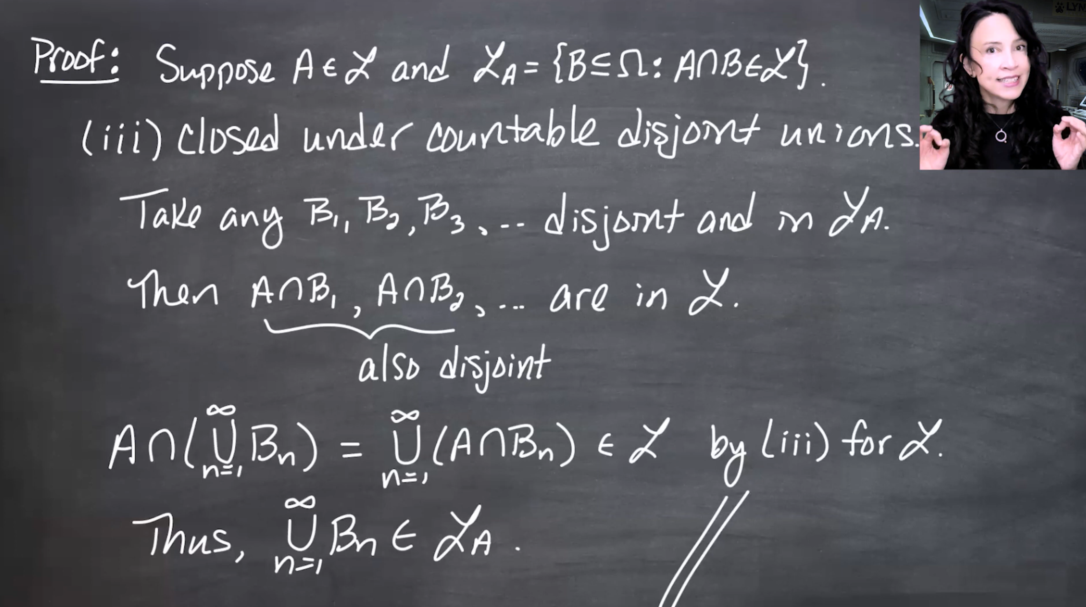
Finally, let B_1,B_2,\ldots be disjoint sets in \mathcal{L}_A. Then A\cap B_1,A\cap B_2,\ldots are disjoint sets in \mathcal{L}. Since \mathcal{L} is a \lambda-system, \bigcup_{n=1}^{\infty}(A\cap B_n) \in\mathcal{L}.
Distributing intersection over union gives
\bigcup_{n=1}^{\infty}(A\cap B_n) = A\cap\left(\bigcup_{n=1}^{\infty}B_n\right).
So \bigcup_{n=1}^{\infty}B_n \in\mathcal{L}_A
155.8 Dynkin’s \pi-\lambda theorem
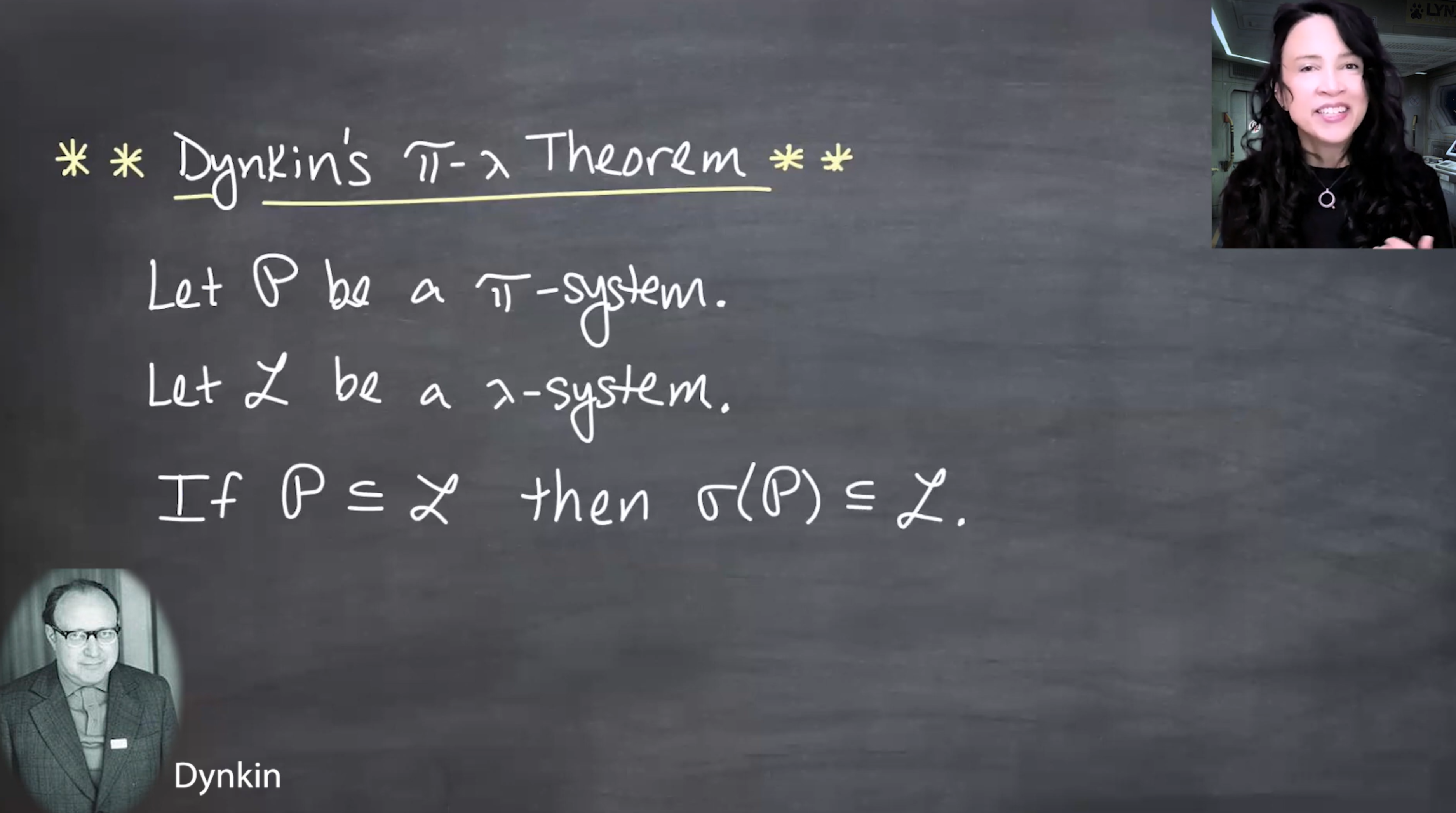
Theorem 155.5 (Dynkin’s \pi-\lambda theorem) Let \mathcal{P} be a \pi-system and let \mathcal{L} be a \lambda-system. If
\mathcal{P}\subseteq\mathcal{L},
then
\sigma(\mathcal{P})\subseteq\mathcal{L}.
Billingsley states this as Theorem 3.2 and uses it immediately for uniqueness of probability measures on generated \sigma-fields (Billingsley 2012, 43–45).
Dynkin’s theorem is a bootstrap: prove a \lambda-system contains a \pi-system, then get the generated \sigma-field for free.
155.8.1 Proof idea
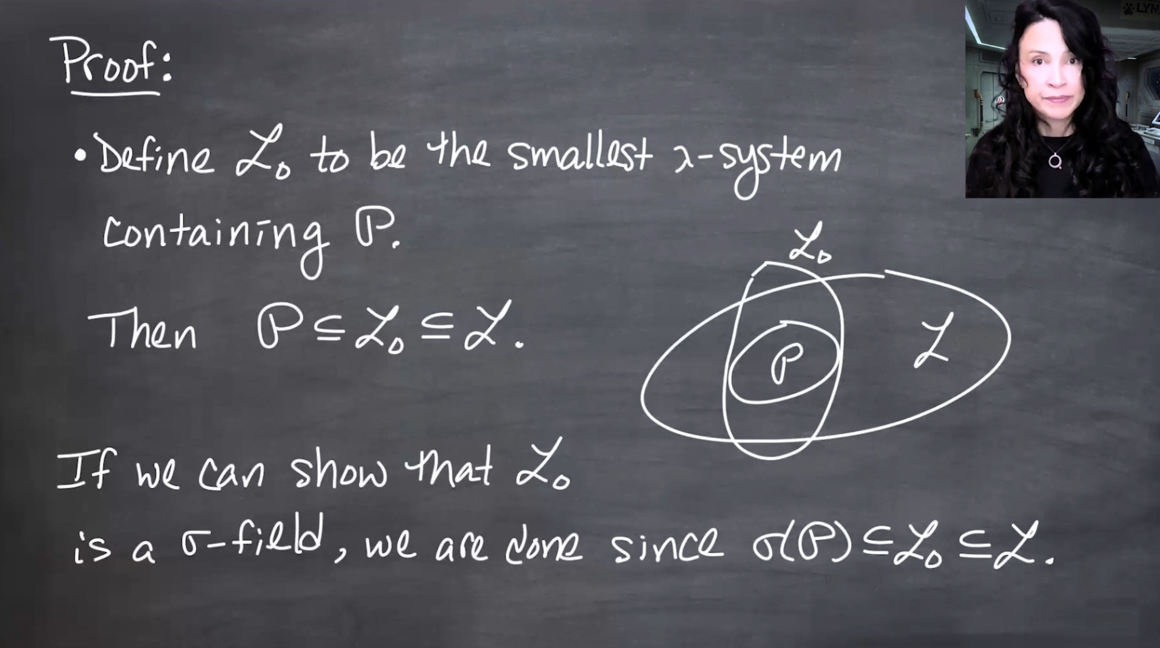
Let \mathcal{L}_0 be the smallest \lambda-system containing \mathcal{P}. Since \mathcal{L} is a \lambda-system containing \mathcal{P},
\mathcal{P} \subseteq \mathcal{L}_0 \subseteq \mathcal{L}.
If we can prove that \mathcal{L}_0 is also a \pi-system, then \mathcal{L}_0 is both a \pi-system and a \lambda-system, hence a \sigma-field. Then minimality of \sigma(\mathcal{P}) gives
\sigma(\mathcal{P}) \subseteq \mathcal{L}_0 \subseteq \mathcal{L}.
So the whole proof reduces to showing:
A,B\in\mathcal{L}_0 \quad\Longrightarrow\quad A\cap B\in\mathcal{L}_0.
155.8.2 Claim 1: intersections with sets in \mathcal{P} preserve \mathcal{P}
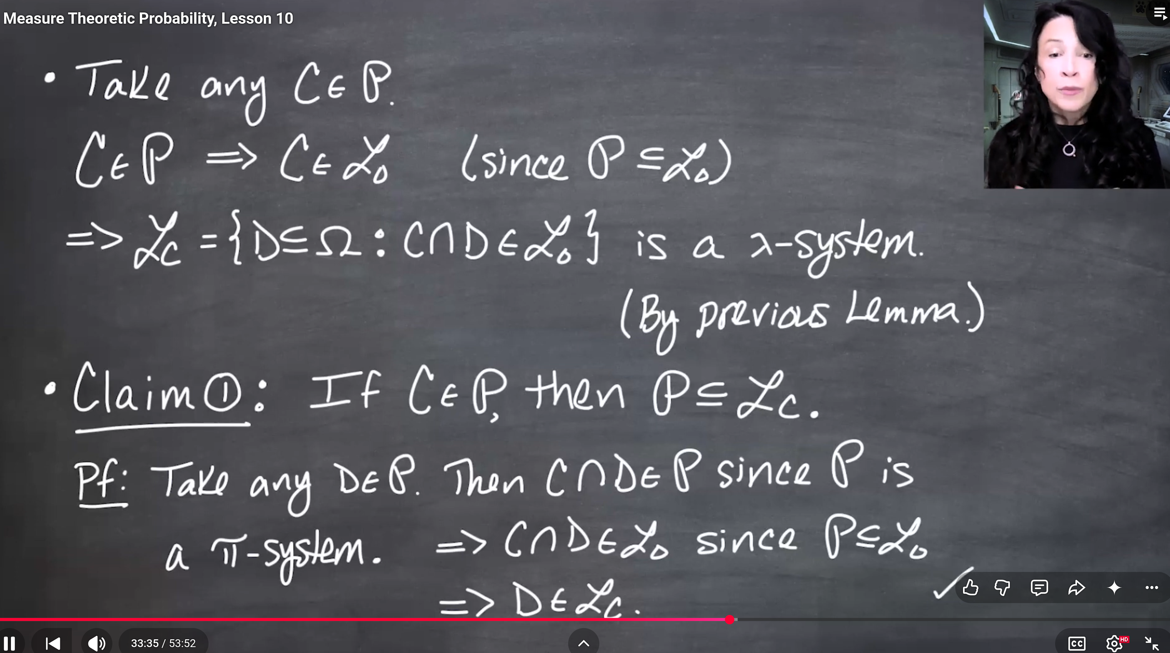
Take C\in\mathcal{P}. Since \mathcal{P}\subseteq\mathcal{L}_0, we also have C\in\mathcal{L}_0. Define
\mathcal{L}_C = \{D\subseteq\Omega:C\cap D\in\mathcal{L}_0\}.
By the section lemma, \mathcal{L}_C is a \lambda-system.
If D\in\mathcal{P}, then because \mathcal{P} is a \pi-system,
C\cap D\in\mathcal{P} \subseteq \mathcal{L}_0.
Therefore D\in\mathcal{L}_C, and hence
\mathcal{P}\subseteq\mathcal{L}_C.
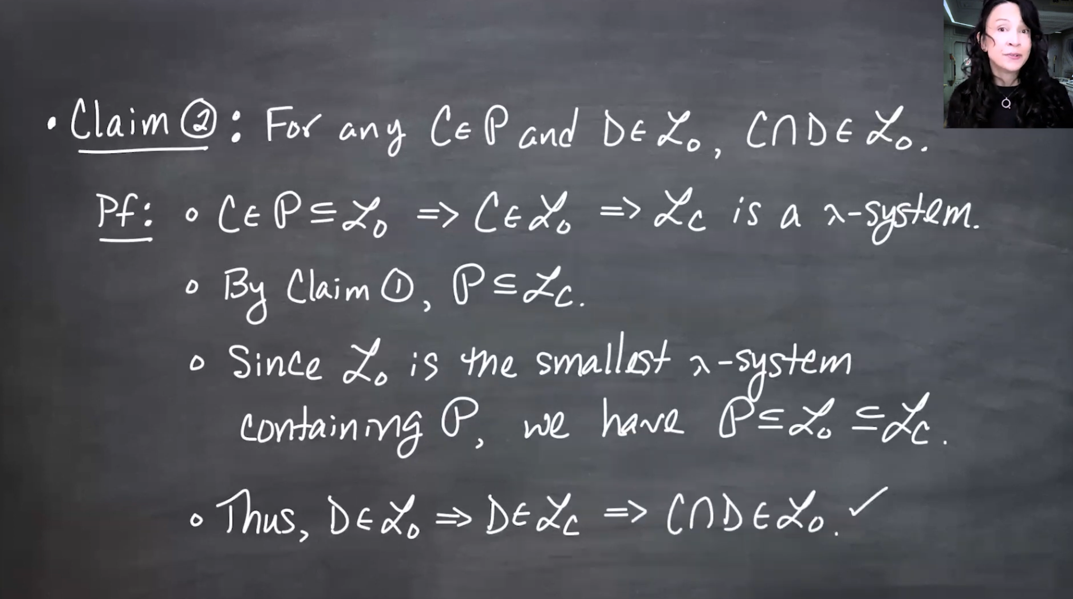
155.8.3 Claim 2: one set from \mathcal{P} and one from \mathcal{L}_0
For C\in\mathcal{P}, Claim 1 gives \mathcal{P}\subseteq\mathcal{L}_C. Since \mathcal{L}_C is a \lambda-system containing \mathcal{P}, minimality of \mathcal{L}_0 gives
\mathcal{L}_0\subseteq\mathcal{L}_C.
Thus if D\in\mathcal{L}_0, then D\in\mathcal{L}_C, which means
C\cap D\in\mathcal{L}_0.
So
C\in\mathcal{P},\ D\in\mathcal{L}_0 \quad\Longrightarrow\quad C\cap D\in\mathcal{L}_0.
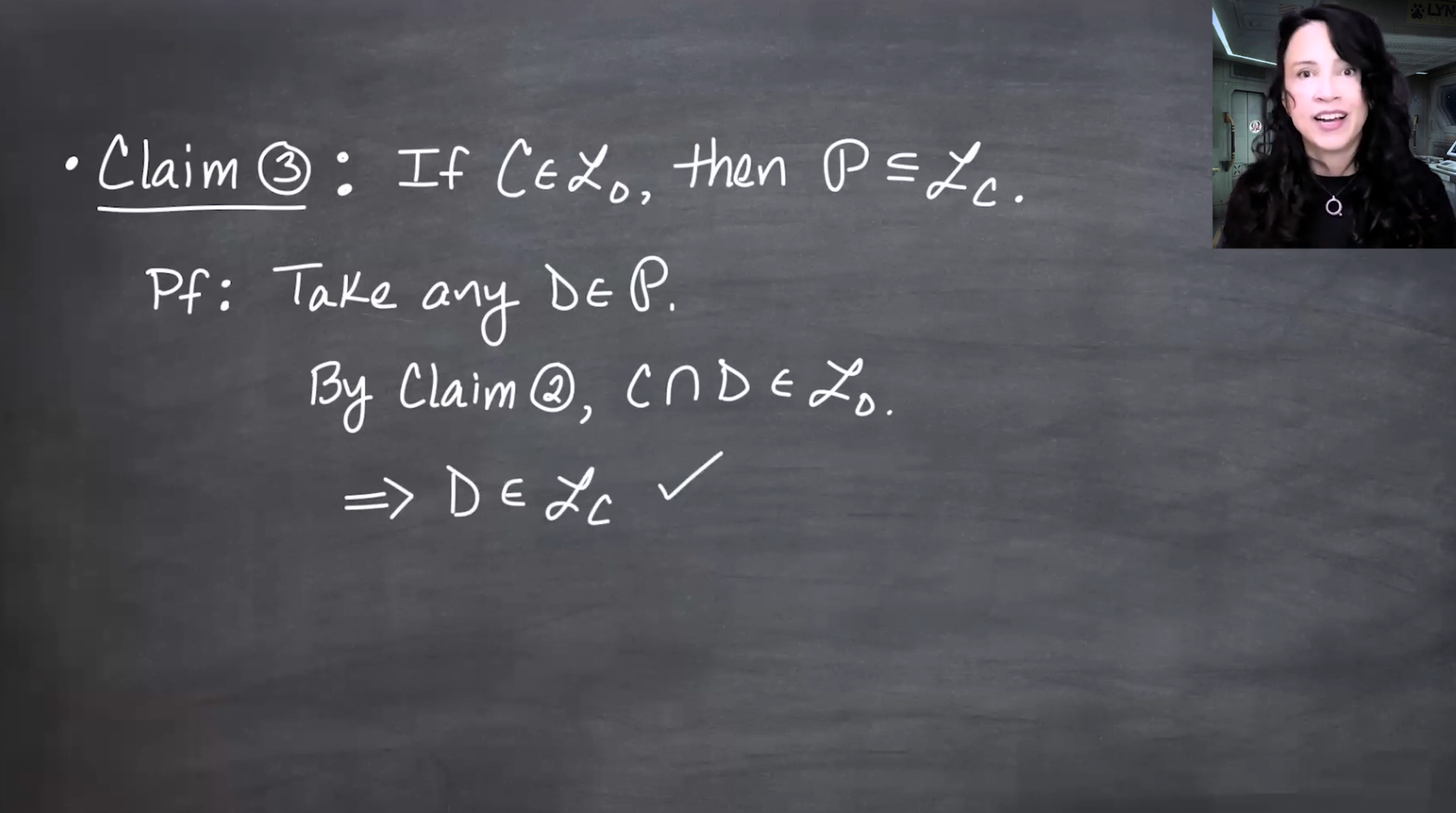
155.8.4 Claim 3: reverse the roles
Now take C\in\mathcal{L}_0. We want to show
\mathcal{P}\subseteq\mathcal{L}_C.
Let D\in\mathcal{P}. By Claim 2, with the \mathcal{P}-set D and the \mathcal{L}_0-set C,
D\cap C \in \mathcal{L}_0.
Since D\cap C=C\cap D, this means D\in\mathcal{L}_C. Hence
\mathcal{P}\subseteq\mathcal{L}_C.
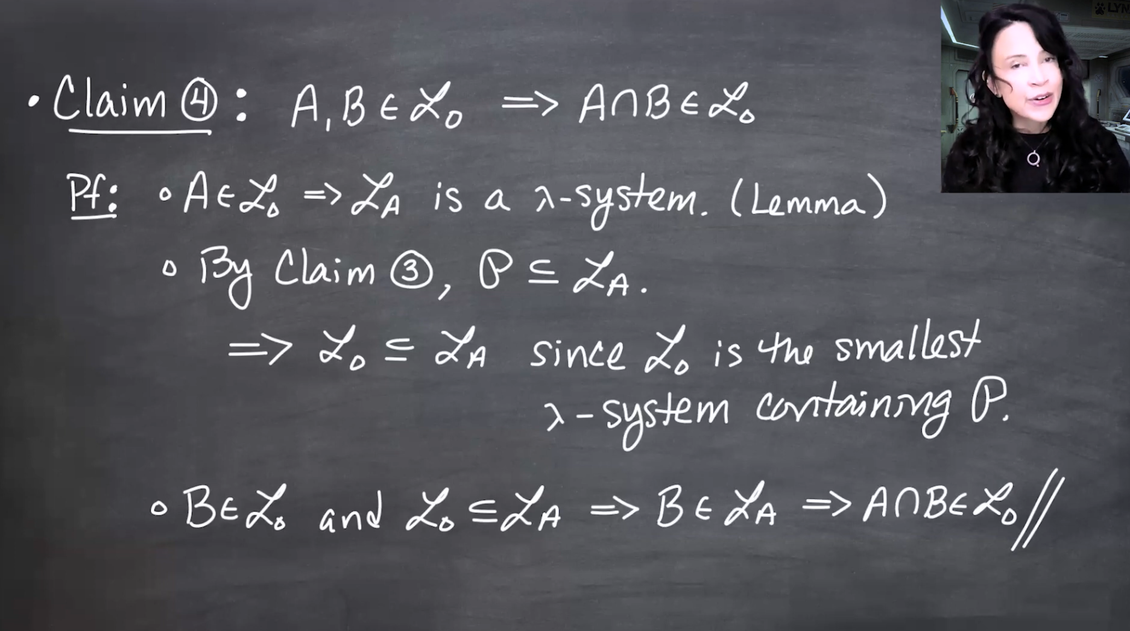
155.8.5 Claim 4: two arbitrary sets from \mathcal{L}_0
Finally take A\in\mathcal{L}_0. By the section lemma, \mathcal{L}_A is a \lambda-system. Claim 3 gives
\mathcal{P}\subseteq\mathcal{L}_A.
Therefore, by minimality,
\mathcal{L}_0\subseteq\mathcal{L}_A.
If B\in\mathcal{L}_0, then B\in\mathcal{L}_A, so
A\cap B\in\mathcal{L}_0.
Thus \mathcal{L}_0 is a \pi-system. Since it is already a \lambda-system, it is a \sigma-field. This proves Dynkin’s \pi-\lambda theorem.
155.9 Independent \pi-systems generate independent \sigma-fields
Now return to the motivation of the lesson.
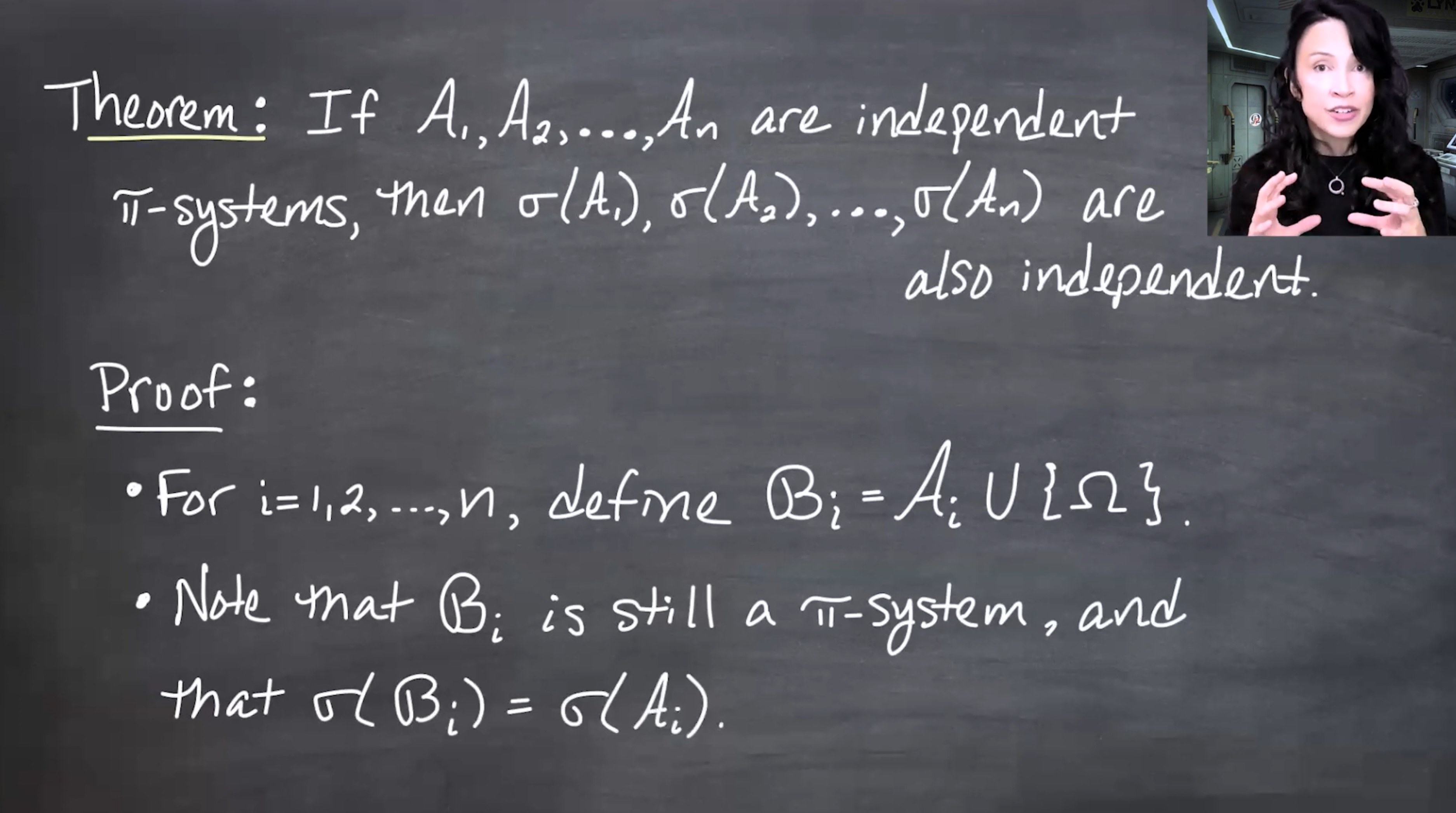
Theorem 155.6 (Independence theorem for generated \sigma-fields) Let
\mathcal{A}_1,\ldots,\mathcal{A}_n
be independent \pi-systems in a probability space (\Omega,\mathcal{F},P). Then
\sigma(\mathcal{A}_1),\ldots,\sigma(\mathcal{A}_n)
are independent.
This is the promised corrected form of the false naive theorem. The extra \pi-system assumption prevents the counterexample pathology.
Define
\mathcal{B}_i = \mathcal{A}_i\cup\{\Omega\}.
Adding \Omega does not break the \pi-system property, because intersecting with \Omega changes nothing. Also,
\sigma(\mathcal{B}_i)=\sigma(\mathcal{A}_i),
since \Omega belongs to every \sigma-field anyway.
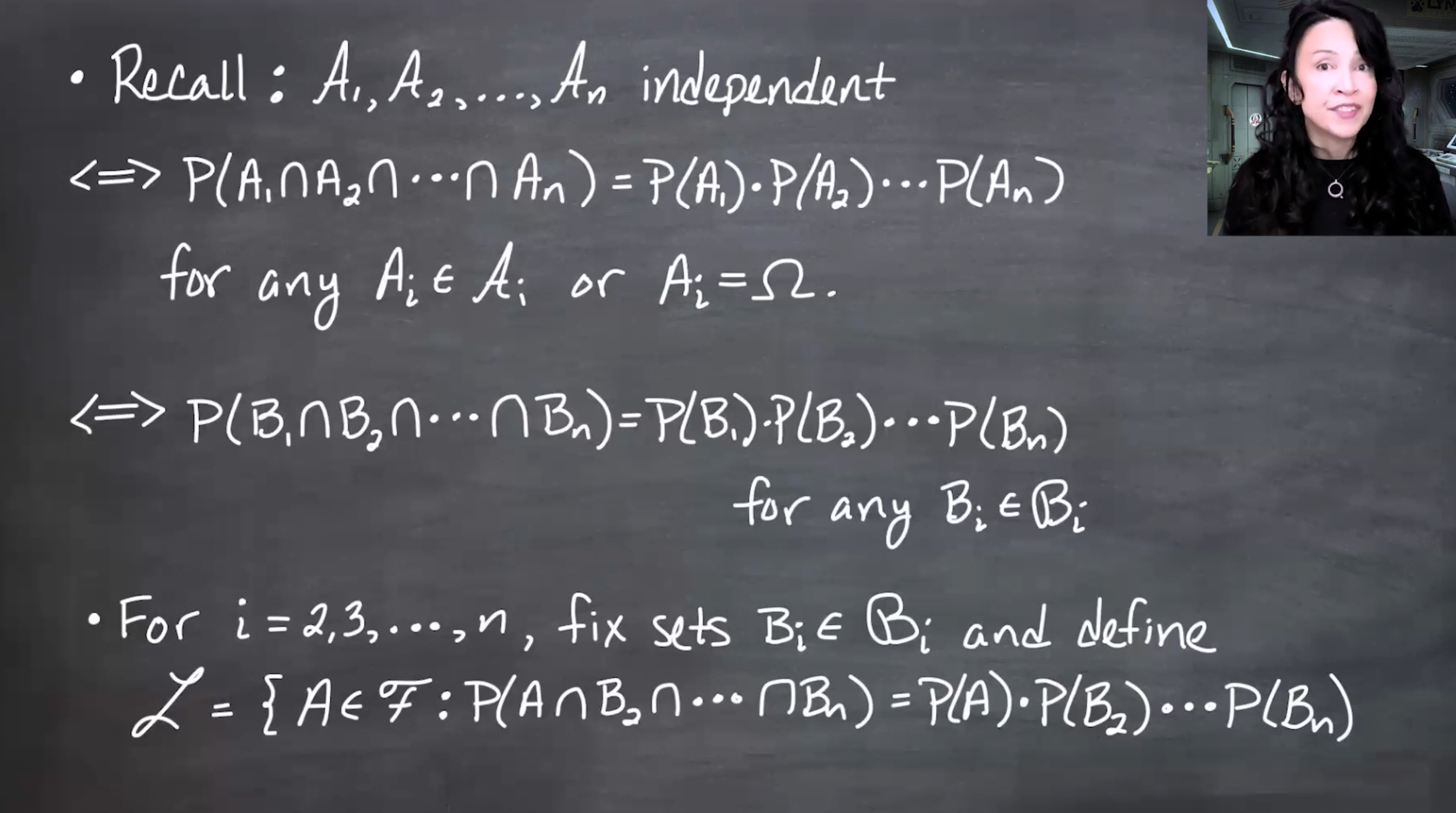
The independence of the original classes is equivalent to saying that for all B_i\in\mathcal{B}_i,
P(B_1\cap\cdots\cap B_n) = \prod_{i=1}^nP(B_i).
Fix arbitrary sets
B_2\in\mathcal{B}_2, \ldots, B_n\in\mathcal{B}_n.
Define
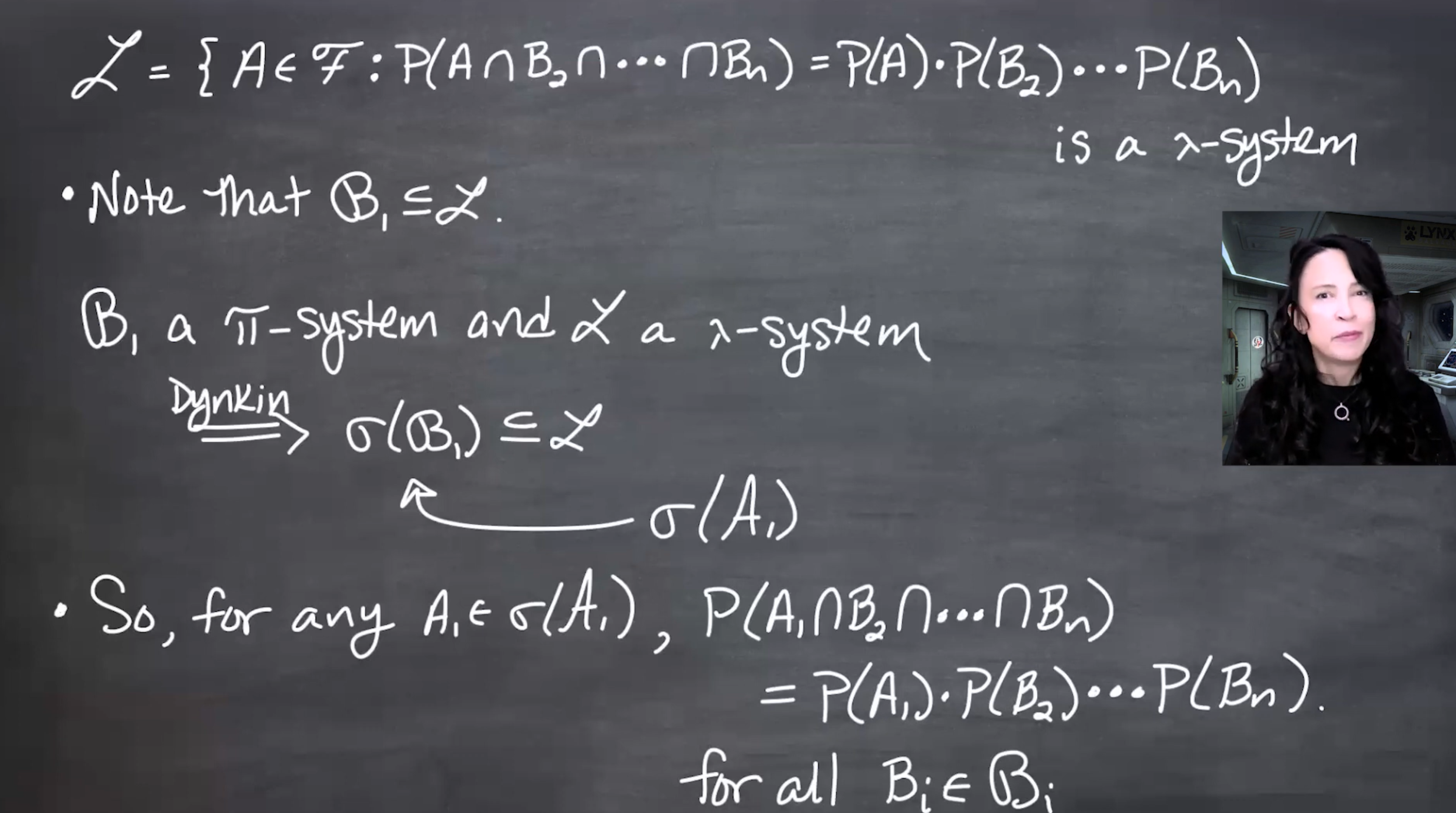
\mathcal{L} = \left\{ A\in\mathcal{F}: P(A\cap B_2\cap\cdots\cap B_n) = P(A)\prod_{i=2}^nP(B_i) \right\}.
The goal is to show that \mathcal{L} is a \lambda-system containing \mathcal{B}_1. Then Dynkin’s theorem gives
\sigma(\mathcal{B}_1) \subseteq \mathcal{L},
which is the first step in replacing \mathcal{B}_1 by \sigma(\mathcal{A}_1).
To put a \sigma on one coordinate, freeze every other coordinate and make the unfrozen coordinate a \lambda-system.
155.9.1 Showing \mathcal{L} is a \lambda-system
First, \Omega\in\mathcal{L} because
P(\Omega\cap B_2\cap\cdots\cap B_n) = P(B_2\cap\cdots\cap B_n) = \prod_{i=2}^nP(B_i) = P(\Omega)\prod_{i=2}^nP(B_i).
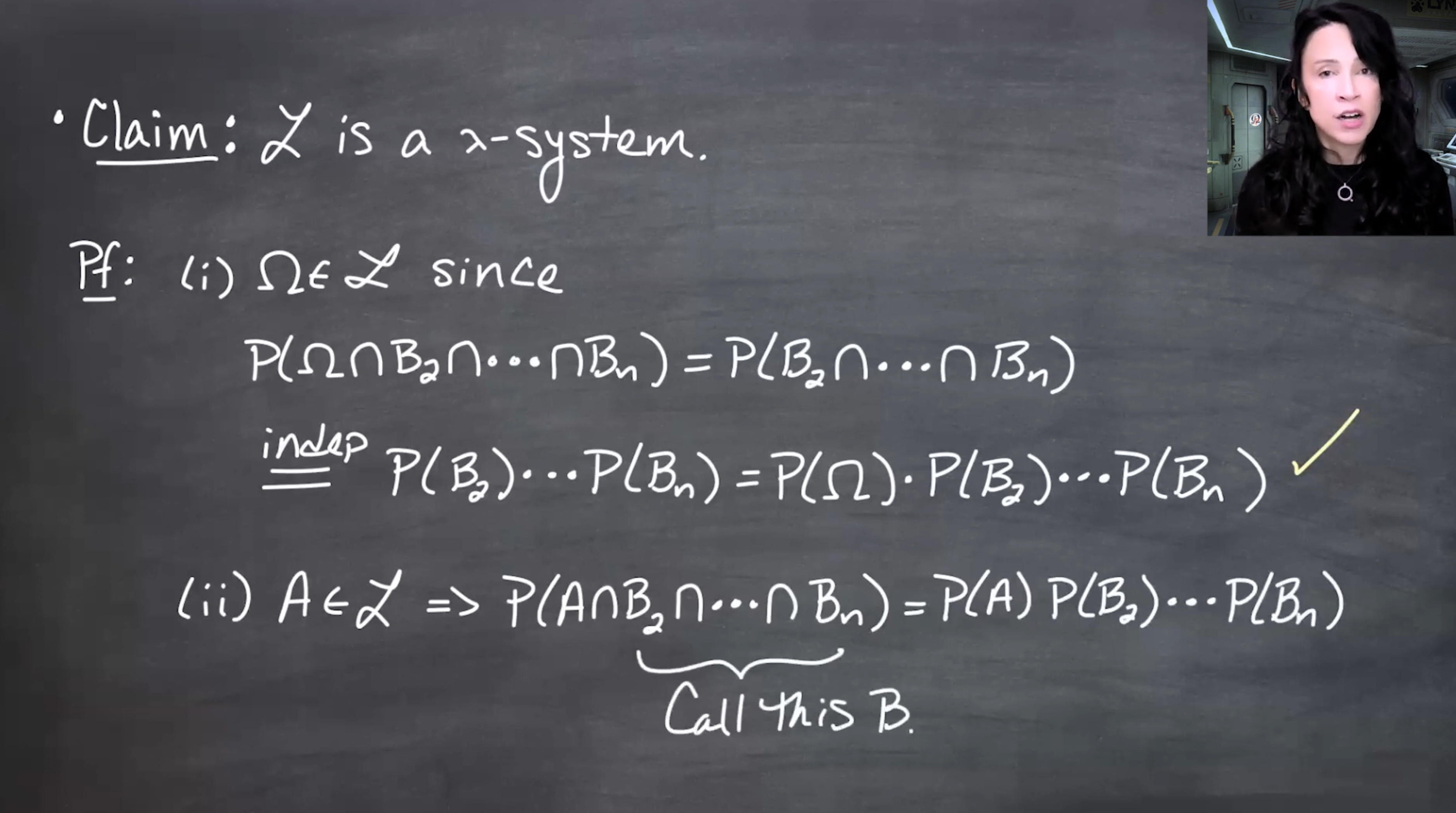
For complements, let A\in\mathcal{L} and abbreviate
B=B_2\cap\cdots\cap B_n.
Then
B=(A\cap B)\cup(A^c\cap B),
and the two pieces are disjoint. By finite additivity,
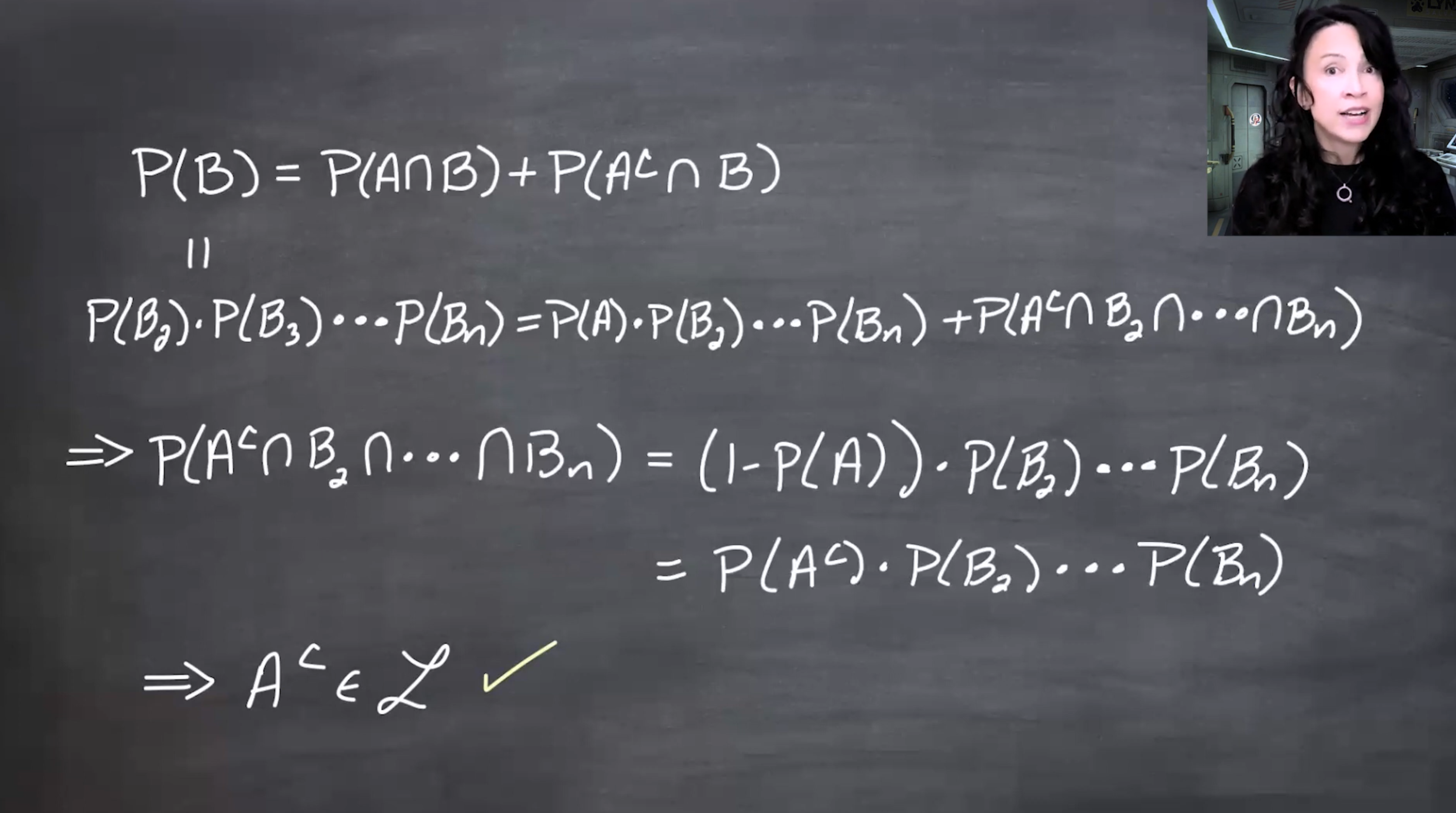
P(B)=P(A\cap B)+P(A^c\cap B).
Because A\in\mathcal{L},
P(A\cap B) = P(A)\prod_{i=2}^nP(B_i).
Also, by independence of B_2,\ldots,B_n,
P(B)=\prod_{i=2}^nP(B_i).
Therefore
P(A^c\cap B) = \left(1-P(A)\right)\prod_{i=2}^nP(B_i) = P(A^c)\prod_{i=2}^nP(B_i).
Thus A^c\in\mathcal{L}.
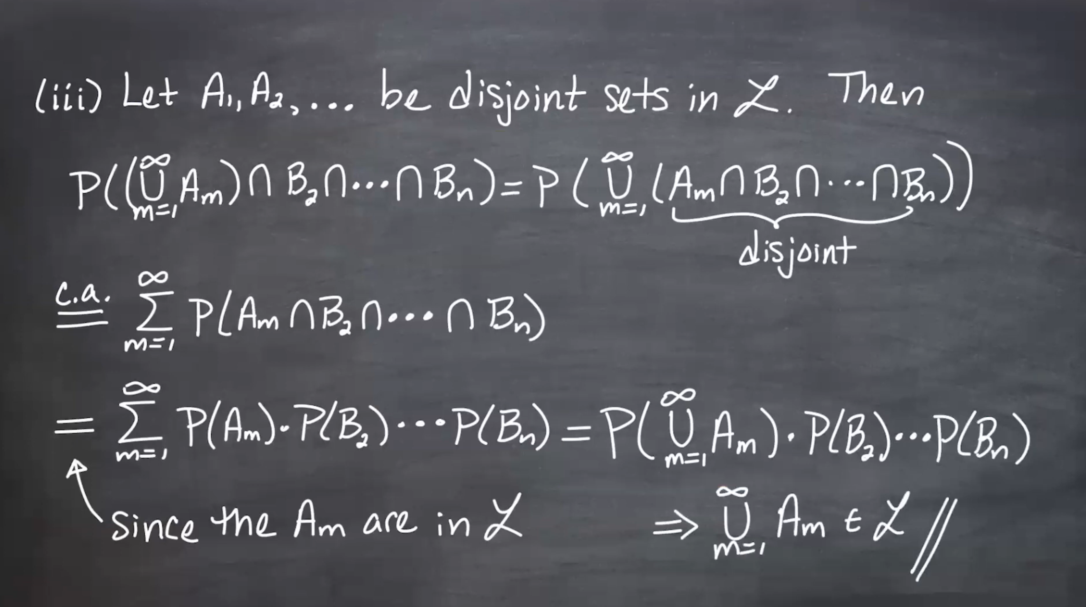
For countable disjoint unions, let A_1,A_2,\ldots\in\mathcal{L} be disjoint. Then the sets
A_m\cap B_2\cap\cdots\cap B_n
are also disjoint. Countable additivity gives
\begin{aligned} P\left(\left(\bigcup_{m=1}^{\infty}A_m\right)\cap B_2\cap\cdots\cap B_n\right) &= P\left(\bigcup_{m=1}^{\infty}(A_m\cap B_2\cap\cdots\cap B_n)\right)\\ &= \sum_{m=1}^{\infty}P(A_m\cap B_2\cap\cdots\cap B_n)\\ &= \sum_{m=1}^{\infty}P(A_m)\prod_{i=2}^nP(B_i)\\ &= \left(\sum_{m=1}^{\infty}P(A_m)\right)\prod_{i=2}^nP(B_i)\\ &= P\left(\bigcup_{m=1}^{\infty}A_m\right)\prod_{i=2}^nP(B_i). \end{aligned}
So
\bigcup_{m=1}^{\infty}A_m\in\mathcal{L}.
155.9.2 Apply Dynkin’s theorem once
Because the original classes are independent, every B_1\in\mathcal{B}_1 satisfies the defining factorization for \mathcal{L}. Hence
\mathcal{B}_1\subseteq\mathcal{L}.
Since \mathcal{B}_1 is a \pi-system and \mathcal{L} is a \lambda-system, Dynkin’s theorem gives
\sigma(\mathcal{B}_1) \subseteq\mathcal{L}.
But \sigma(\mathcal{B}_1)=\sigma(\mathcal{A}_1), so for any
A_1\in\sigma(\mathcal{A}_1),
and any fixed B_2\in\mathcal{B}_2,\ldots,B_n\in\mathcal{B}_n,
P(A_1\cap B_2\cap\cdots\cap B_n) = P(A_1)\prod_{i=2}^nP(B_i).
Thus
\sigma(\mathcal{A}_1),\mathcal{B}_2,\ldots,\mathcal{B}_n
are independent.
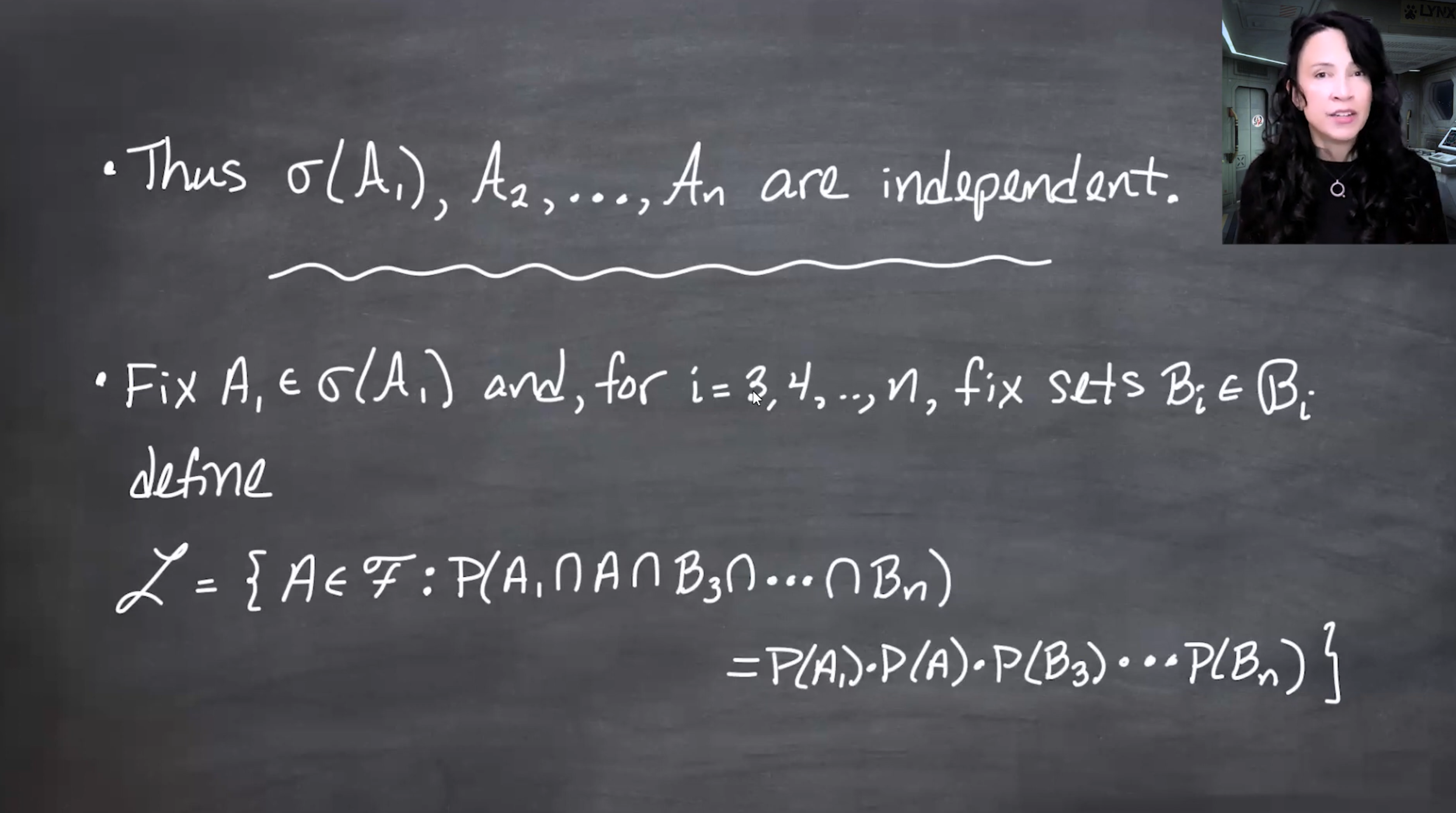
155.9.3 Iterate the argument
Now fix
A_1\in\sigma(\mathcal{A}_1), \qquad B_3\in\mathcal{B}_3, \ldots, B_n\in\mathcal{B}_n,
and define a new class
\mathcal{L} = \left\{ A\in\mathcal{F}: P(A_1\cap A\cap B_3\cap\cdots\cap B_n) = P(A_1)P(A)\prod_{i=3}^nP(B_i) \right\}.
The same proof shows that this new \mathcal{L} is a \lambda-system containing \mathcal{B}_2. Dynkin’s theorem gives
\sigma(\mathcal{B}_2) \subseteq \mathcal{L},
so \mathcal{B}_2 can be upgraded to \sigma(\mathcal{A}_2).
Repeating the argument for \mathcal{A}_3,\ldots,\mathcal{A}_n yields
\sigma(\mathcal{A}_1), \sigma(\mathcal{A}_2), \ldots, \sigma(\mathcal{A}_n)
mutually independent.
For an infinite collection of independent \pi-systems, the result follows by applying the finite theorem to every finite subcollection. This works because independence of an infinite family is defined by independence of all finite subfamilies.
The infinite-family version follows because independence is checked on finite subfamilies.
155.10 Takeaway
Dynkin’s \pi-\lambda theorem is a minimality machine. It says that once a \lambda-system contains a \pi-system, it must contain everything generated from that \pi-system as a \sigma-field.
The lesson uses that machine twice:
- Abstractly, to prove the theorem itself by showing the minimal \lambda-system over a \pi-system is also a \pi-system.
- Probabilistically, to prove that independent \pi-systems remain independent after generating \sigma-fields.
This is also why \lambda-systems are tuned to probability: their closure condition is countable additivity over disjoint unions, which is the central operation for probability measures (Billingsley 2012, 45).