127.1 Illustrating the time-domain response
127.1.1 Deconstructing the matrix exponential
- Have seen the key role of e^{At} in the solution for x(t).
- Impacts the system response, but need more insight.
- Consider what happens if the matrix A is diagonalizable, that is, there exists a matrix T such that T^{-1}AT = \Delta is diagonal. Then,
\begin{aligned} e^{At} &= I + At + \frac{1}{2!} A^2t^2 + \frac{1}{3!} A^3t^3 + \cdots \\ &= I + T \Delta T^{-1}t + \frac{1}{2!}T \Delta^2 T^{-1}t^2 + \frac{1}{3!}T \Delta^3 T^{-1}t^3 + \cdots \\ &= T \left( I + \Delta t + \frac{1}{2!} \Delta^2 t^2 + \frac{1}{3!} \Delta^3 t^3 + \cdots \right) T^{-1} \\ &= T e^{\Delta t} T^{-1} \end{aligned}
and
e^{\Delta t} = \text{diag} \left( e^{\lambda_1 t}, e^{\lambda_2 t}, \ldots, e^{\lambda_n t} \right)
127.1.2 How to find the transformation matrix
- Much simpler form for the exponential, but how to find T, \Delta ?
- Write T^{-1}AT = \Delta as T^{-1}A = \Delta T^{-1} with
T^{-1} = \begin{bmatrix} w_1^T \\ w_2^T \\ \vdots \\ w_n^T \end{bmatrix} \qquad w^T_j \text{ are the rows of } T^{-1}
- We have: w^T_i A = \lambda_i w^T_i; so w_i is a left eigenvector of A.
- Can also write T^{-1}AT = \Delta as AT = \Delta T with
T = \begin{bmatrix} v_1 & v_2 & \cdots & v_n \end{bmatrix}
i.e v_j are the columns of T. - We have Av_i = \lambda_i v_i, so v_i is a right eigenvector of A. Also, since T^{-1}T = I, we have that w^T_i v_j = \delta_{i,j}
127.1.3 How the deconstruction simplifies things
So T comprises the eigenvectors of A. How does this help?
e^{At} = Te^{\Delta t} T^{-1} = \begin{bmatrix} v_1, v_2, \ldots, v_n \end{bmatrix} \begin{bmatrix} e^{\lambda_1 t} & 0 & \cdots & 0 \\ 0 & e^{\lambda_2 t} & \cdots & 0 \\ \vdots & \vdots & \ddots & \vdots \\ 0 & 0 & \cdots & e^{\lambda_n t} \end{bmatrix} \begin{bmatrix} w_1^T \\ w_2^T \\ \vdots \\ w_n^T \end{bmatrix} = \sum _{}^n e^{\lambda_i t} v_i w_i^T
- Very simple form, which can be used to develop intuition about dynamic response:
x(t) = e^{At} x(0) =T e^{\Delta t} T^{-1} x(0) = \sum _{}^n e^{\lambda_i t} v_i w_i^T x(0).
- Notice that the only time-varying components are e^{\lambda_i t} , which are then multiplied by constant matrices so that the states are linear combinations of e^{\lambda_i t} .
127.1.4 Visualizing e^{\lambda_i t}
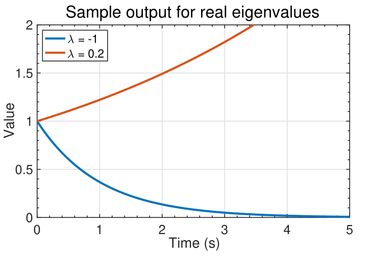
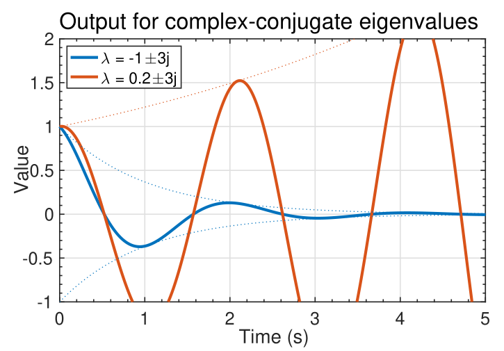
- The signal e^{\lambda_it} can take on several different characteristics, as shown in the figures below.
- If \lambda_i is real, we observe a smooth monotonically growing or decaying signal.
- If \lambda_i occur in complex-conjugate pairs, the output is of the pair is of the form e^{\lambda_i t} \cos(\lambda_i t) : a cosine with an exponential “envelope.”
127.1.5 An example to illustrate the complexity
Consider again: \sum _{i=1}^n e^{\lambda_i t} v_i (w^T_i x(0))
The state x(t) = e^{At} x(0) =T e^{\Delta t} T^{-1} x(0) = \sum _{}^n e^{\lambda_i t} v_i w_i^T x(0) is a linear combination of the modes e^{\lambda_i t} v_i.
The left eigenvectors w_i^T decompose the initial state x(0) into modal coordinates w^T_i x(0).
The modes e^{\lambda_i t} propagate the modal components forward in time.
The output y(t) = C x(t) is
Can be expressed as a linear combination of modes: v_i e^{\lambda_i t}.
Left eigenvectors decompose x(0) into modal coordinates w^T_i x(0).
e^{\lambda_i t} propagates mode forward in time.
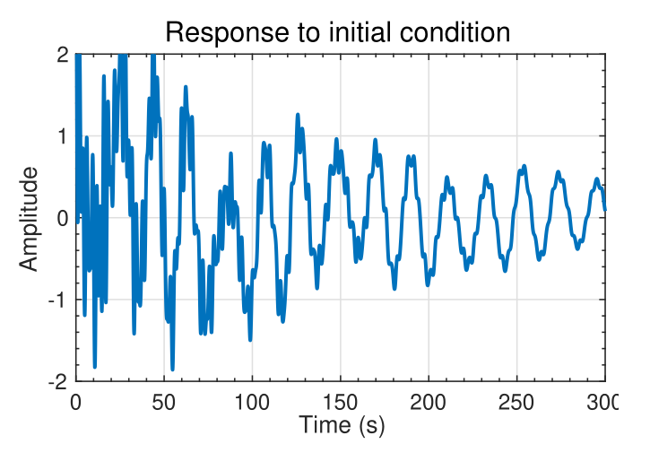
EXAMPLE: Consider a specific system with x(t) \in R^{16 \times 1}; \dot{y}(t) \in R (16-state, 1-output):Px(t) = Ax(t) \dot{y}(t) = C x(t)
A lightly damped system, for which typical output to initial conditions is shown.
Waveform is complicated. Appears random
127.1.6 Now we see the underlying simplicity
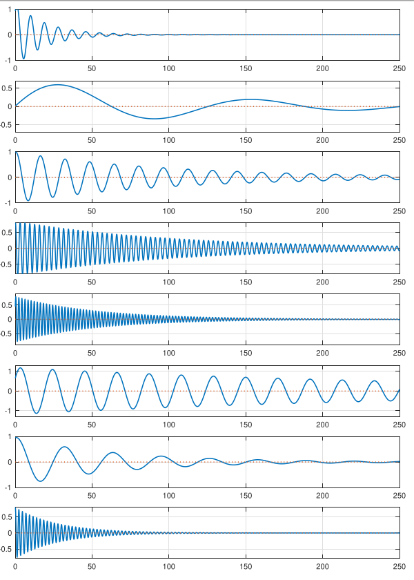
- However, the solution can be decomposed into much simpler modal components.
- The waveforms to the left show e^{\lambda_i t} for complex-conjugate pairs \lambda_i,\lambda_i^* summed together.
- All are decaying sinusoids with different magnitudes, frequencies, and phase shifts.
- When summed together, the result appears complicated; but the individual components of the response are simple.
127.1.7 Summary
- The matrix exponential is key to understanding the response of a state-space model.
- As it’s been a while since I saw the matrix exponent, it’s worthwhile to refresh my intuition regarding what it looks like.1
- You have learned that we can usually write e^{At} = T e^{\Delta t} T^{-1}, where the columns of T are the eigenvectors of A.
- All the dynamics are contained in e^{\Delta t} , which turn out to be the standard scalar exponentials of (possibly complex) \lambda_i t terms.
- So, the matrix exponential is a linear sum of exponentially-enveloped sinusoids.
- The frequencies of the sinusoids are the eigenvalues of A. The eigenvectors specify the relative weighting of each component to the overall output.
Actually this is the first time I see the matrix exponential being used in an application↩︎