Last lesson introduced measurable sets through the idea of a field and a \sigma-field. This lesson asks how to generate a \sigma-field from a smaller starting collection of sets, then applies that idea to construct the Borel \sigma-field on \mathbb{R}.
147.1 Lesson 2: Borel Sets
This video reviews fields and \sigma-fields, defines the \sigma-field generated by a collection of sets, proves that intersections of \sigma-fields are again \sigma-fields, and introduces the Borel \sigma-field on the real line.
147.1.1 Recap
A measure is a function that takes a set as input and returns a number. For ordinary geometric examples, Lebesgue measure behaves like length, area, or volume. The formal definition of measure comes next; for now the focus is on which sets are allowed to be measured.
A field is a collection of subsets of \Omega that:
- contains \Omega,
- is closed under complements,
- is closed under finite unions.
A \sigma-field strengthens the third condition: it is closed under countable unions, not just finite unions. Therefore every \sigma-field is a field, but not every field is a \sigma-field.
The motivating question is:
Starting with a collection of sets, can we add exactly the sets needed to make it a \sigma-field?
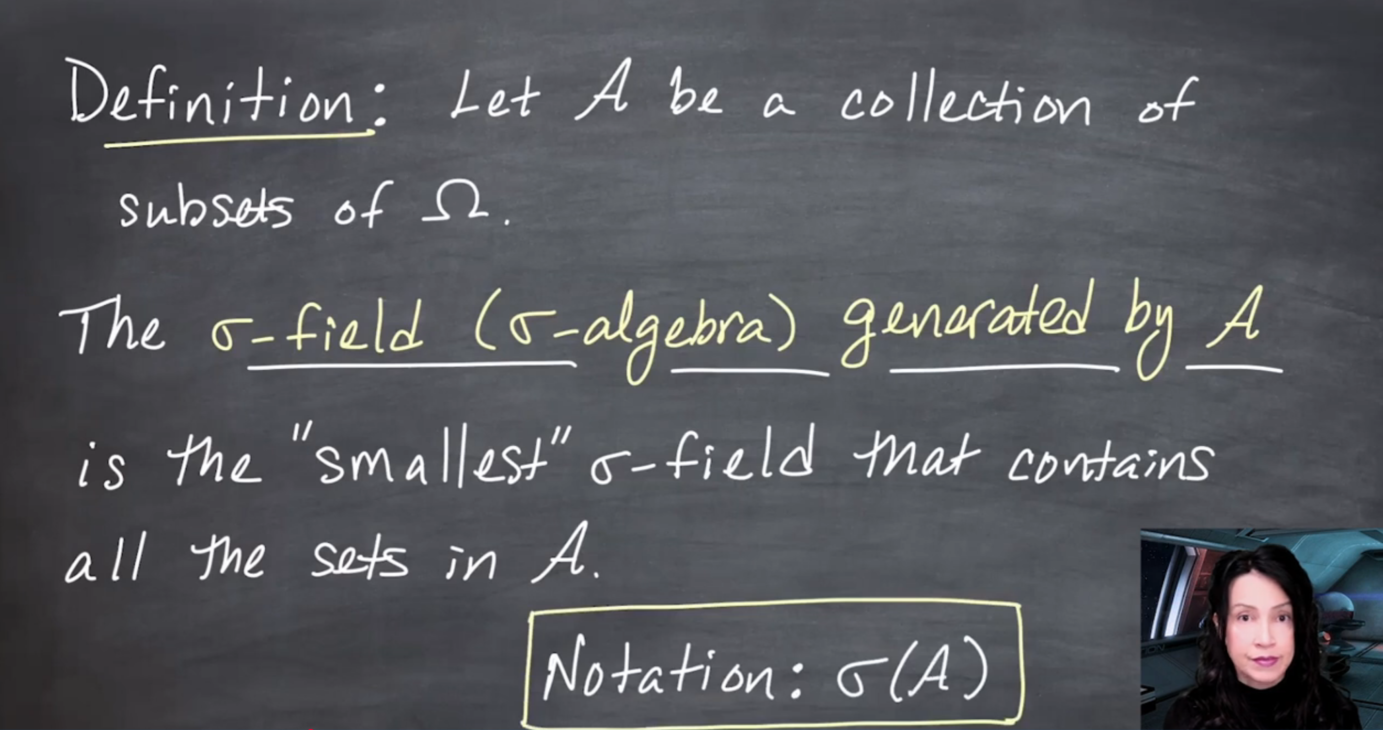
The answer is yes. If \mathcal{A} is a collection of subsets of \Omega, we can generate the smallest \sigma-field containing all sets in \mathcal{A}.
Definition 147.1 (\sigma-field generated by a collection of sets) Given a collection of sets \mathcal{A} \subseteq \mathcal{P}(\Omega), the \sigma-field generated by \mathcal{A} is the smallest \sigma-field that contains \mathcal{A}.
Notation:
\sigma(\mathcal{A}).
Intuitively, \sigma(\mathcal{A}) is what we get by starting with \mathcal{A} and forcing closure under complements and countable unions, while adding no unnecessary sets.
147.1.2 A first minimality fact
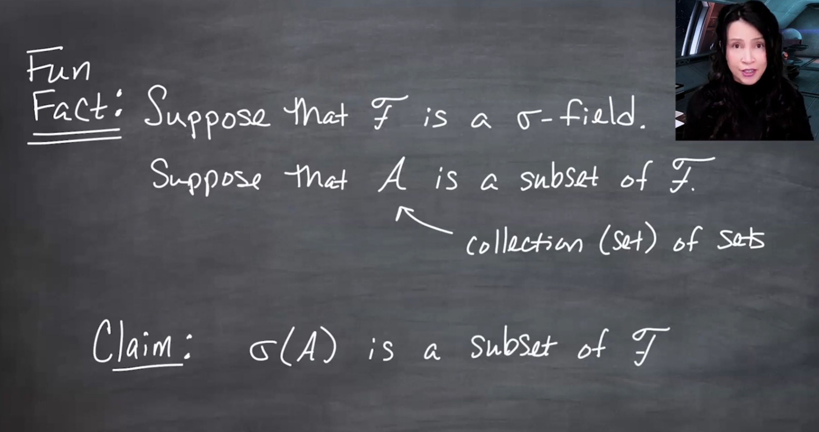
If \mathcal{F} is a \sigma-field and \mathcal{A} \subseteq \mathcal{F}, then
\sigma(\mathcal{A}) \subseteq \mathcal{F}.
This is the key minimality property: once \mathcal{F} already contains the generating collection \mathcal{A}, the smallest \sigma-field containing \mathcal{A} cannot be larger than \mathcal{F}.
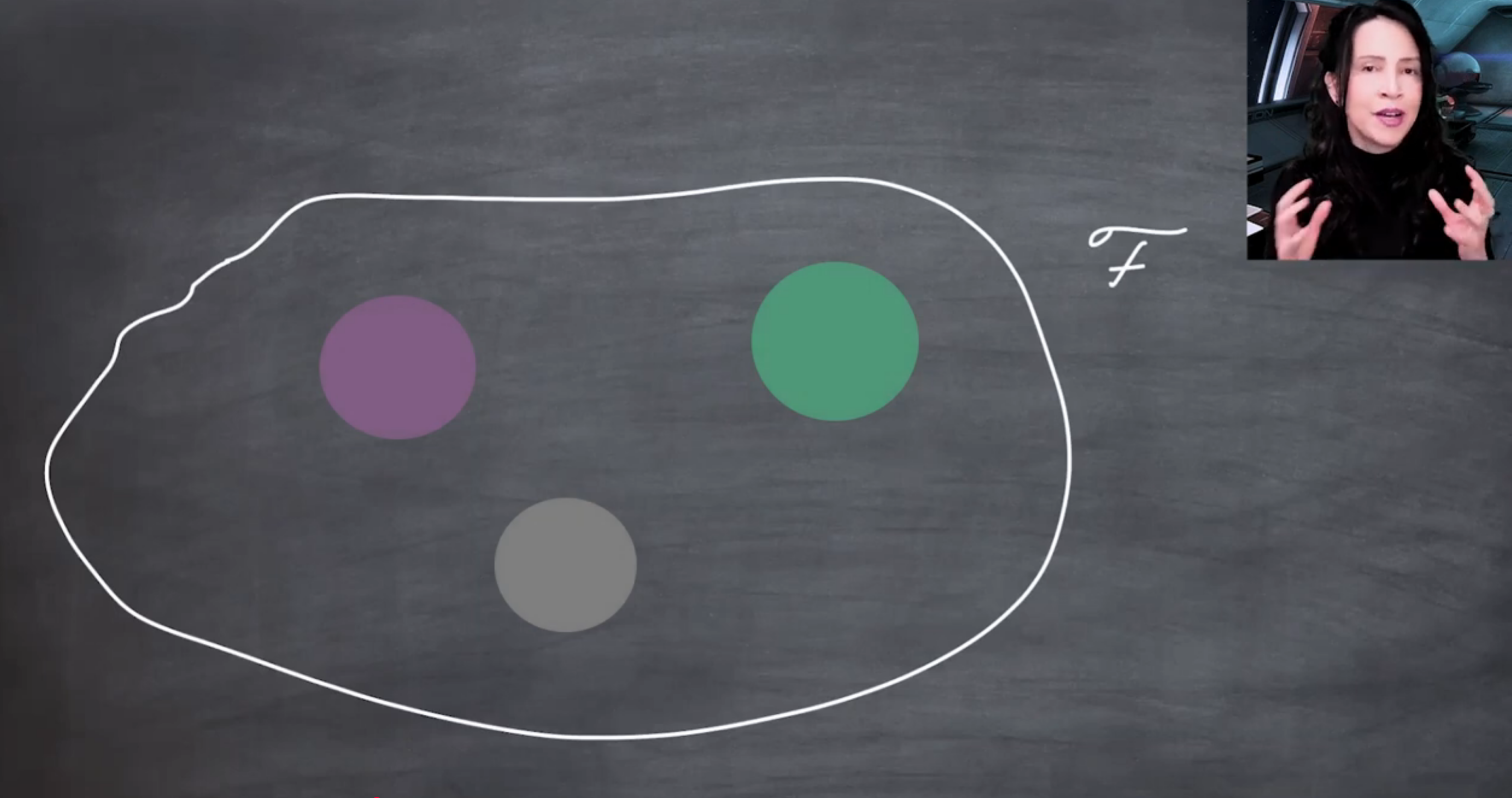
In the picture, \mathcal{F} is a \sigma-field: a collection whose elements are themselves subsets of \Omega.
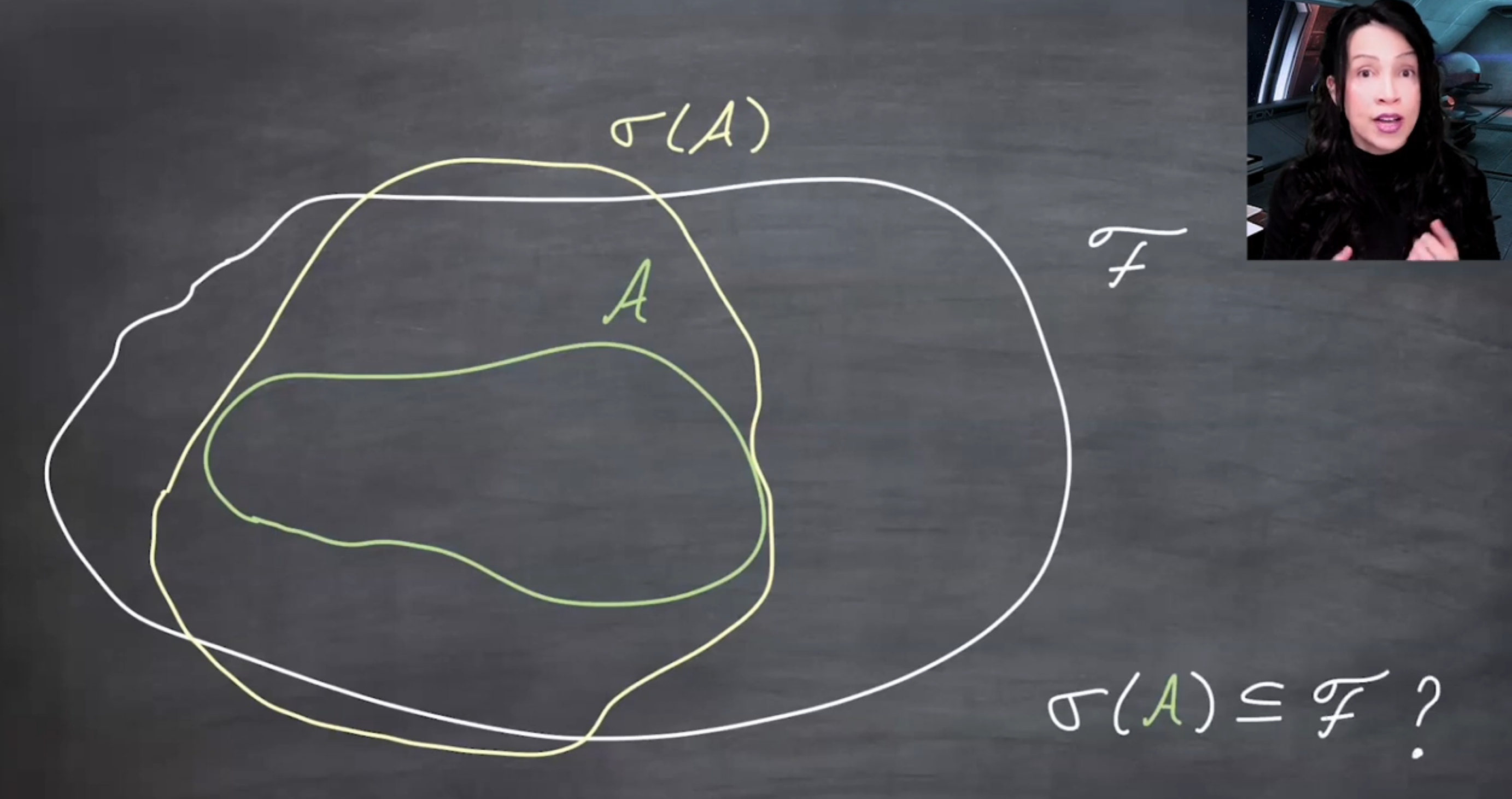
Suppose we draw \sigma(\mathcal{A}) as partly outside \mathcal{F}. That picture cannot be right, because \mathcal{F} itself is one of the \sigma-fields containing \mathcal{A}.
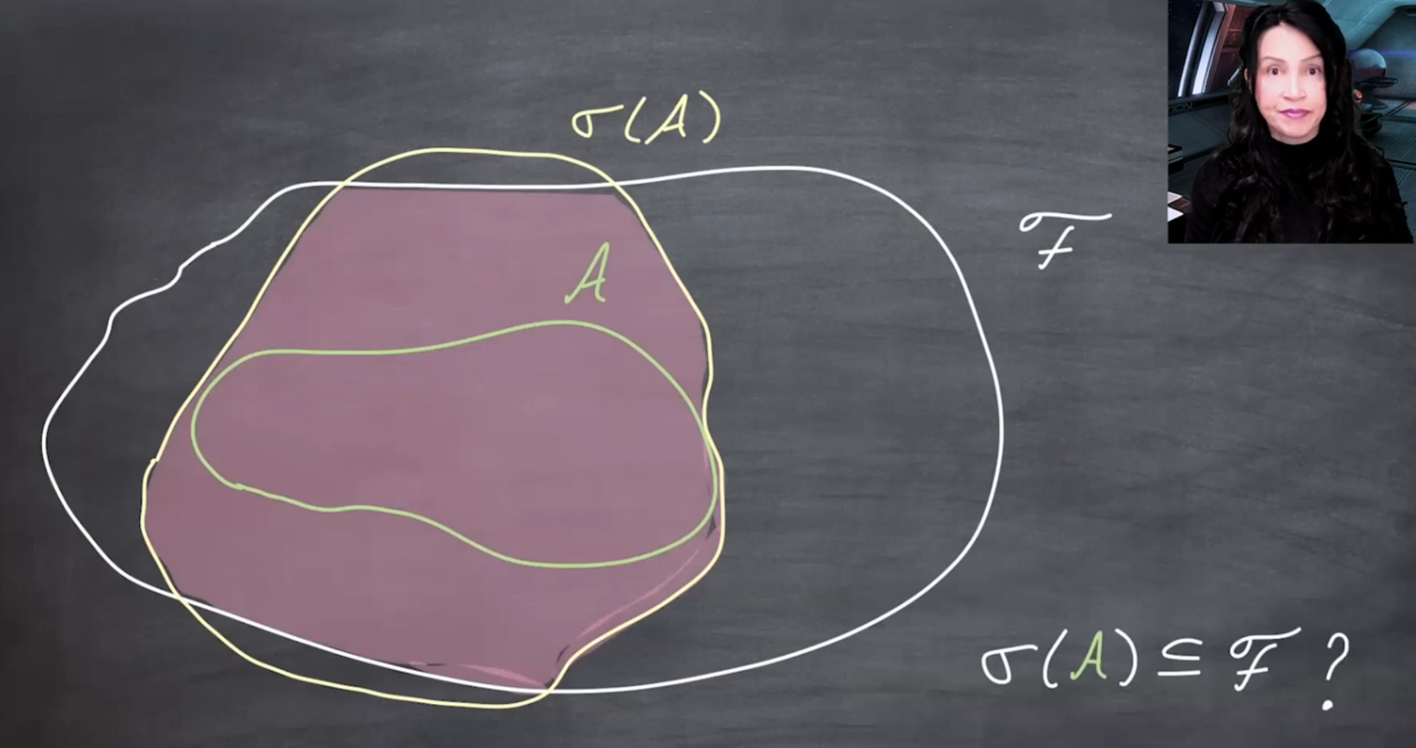
The contradiction is this: if \sigma(\mathcal{A}) escaped outside \mathcal{F}, then
\sigma(\mathcal{A}) \cap \mathcal{F}
would still be a \sigma-field containing \mathcal{A}, but it would be smaller than \sigma(\mathcal{A}). That contradicts the definition of \sigma(\mathcal{A}) as the smallest such \sigma-field.
147.1.3 Intersections of \sigma-fields
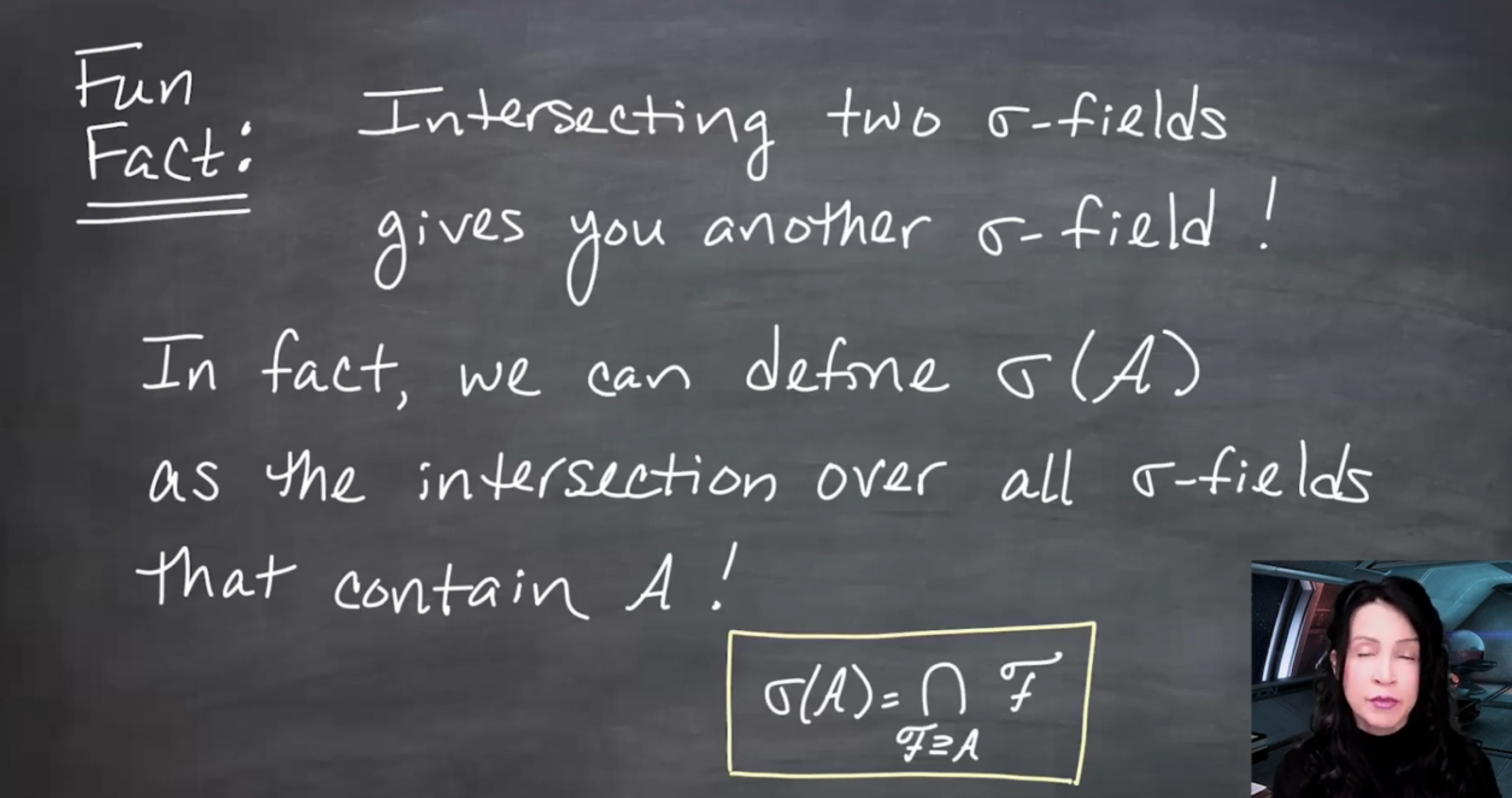
The formal definition is:
\sigma(\mathcal{A}) = \bigcap \{\mathcal{F}: \mathcal{F} \text{ is a } \sigma\text{-field on } \Omega \text{ and } \mathcal{A} \subseteq \mathcal{F}\}.
This definition is meaningful because at least one such \sigma-field always exists: the power set \mathcal{P}(\Omega).
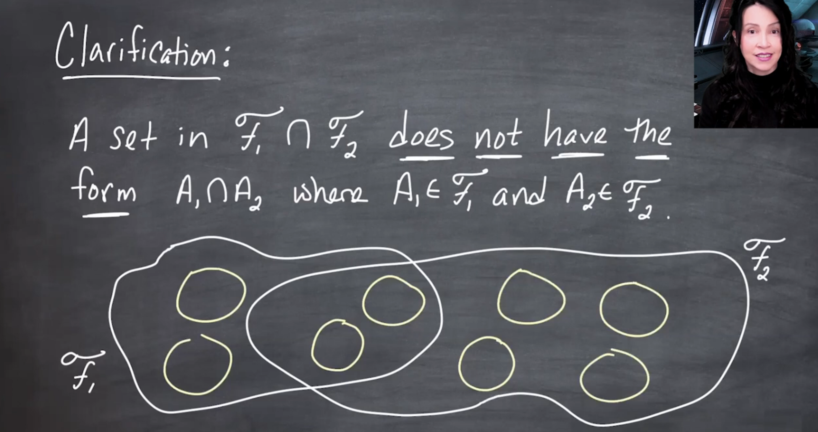
Important distinction: when we write \mathcal{F}_1 \cap \mathcal{F}_2, we are intersecting collections of sets. A set in \mathcal{F}_1 \cap \mathcal{F}_2 is a whole set that belongs to both \mathcal{F}_1 and \mathcal{F}_2. It is not necessarily of the form A_1 \cap A_2.
Proposition 147.1 (Intersection of two \sigma-fields) If \mathcal{F}_1 and \mathcal{F}_2 are \sigma-fields on the same underlying set \Omega, then
\mathcal{F}_1 \cap \mathcal{F}_2
is also a \sigma-field on \Omega.
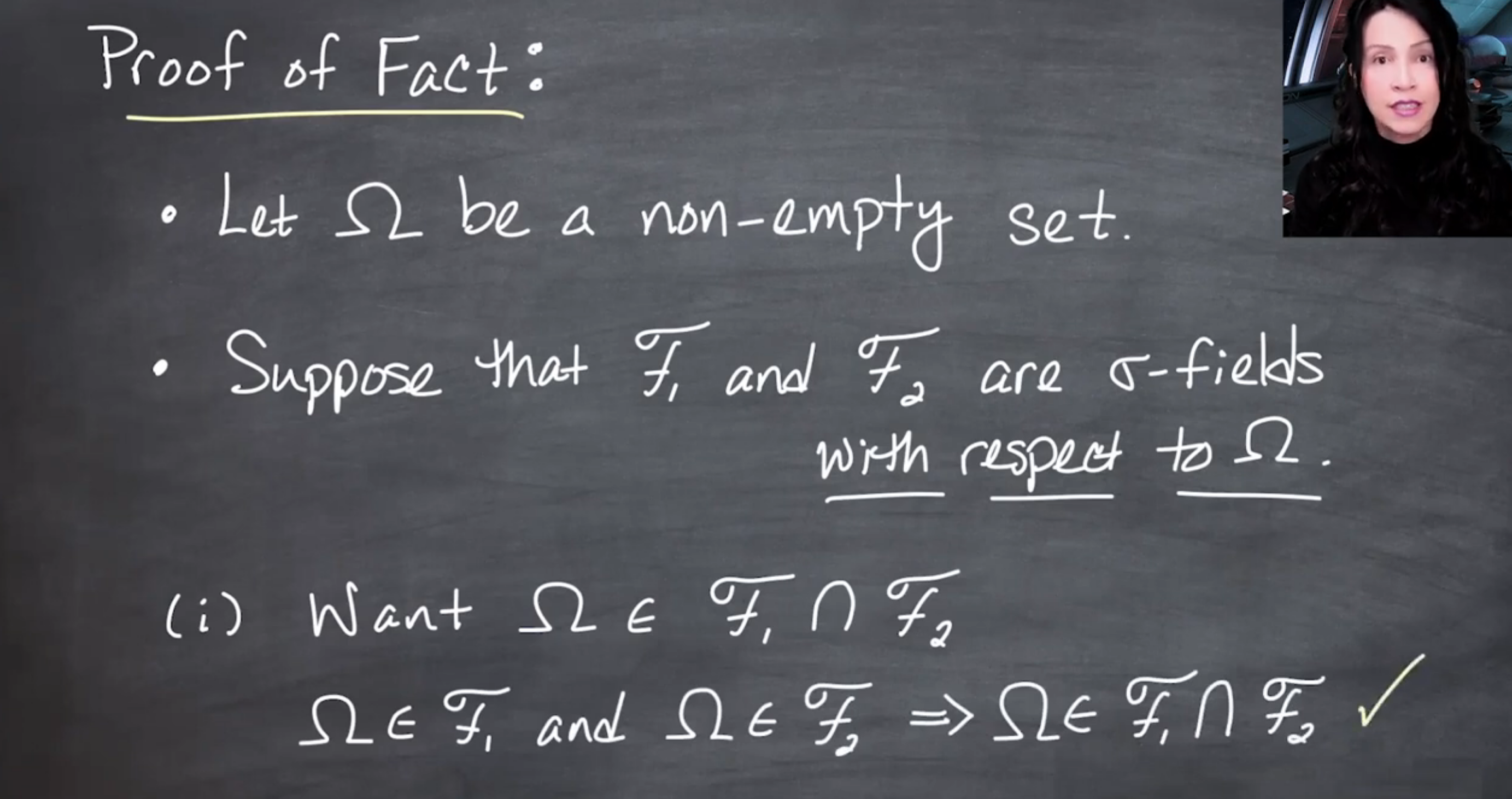
First, since \mathcal{F}_1 and \mathcal{F}_2 are both \sigma-fields on \Omega,
\Omega \in \mathcal{F}_1 \quad \text{and} \quad \Omega \in \mathcal{F}_2.
Therefore,
\Omega \in \mathcal{F}_1 \cap \mathcal{F}_2.
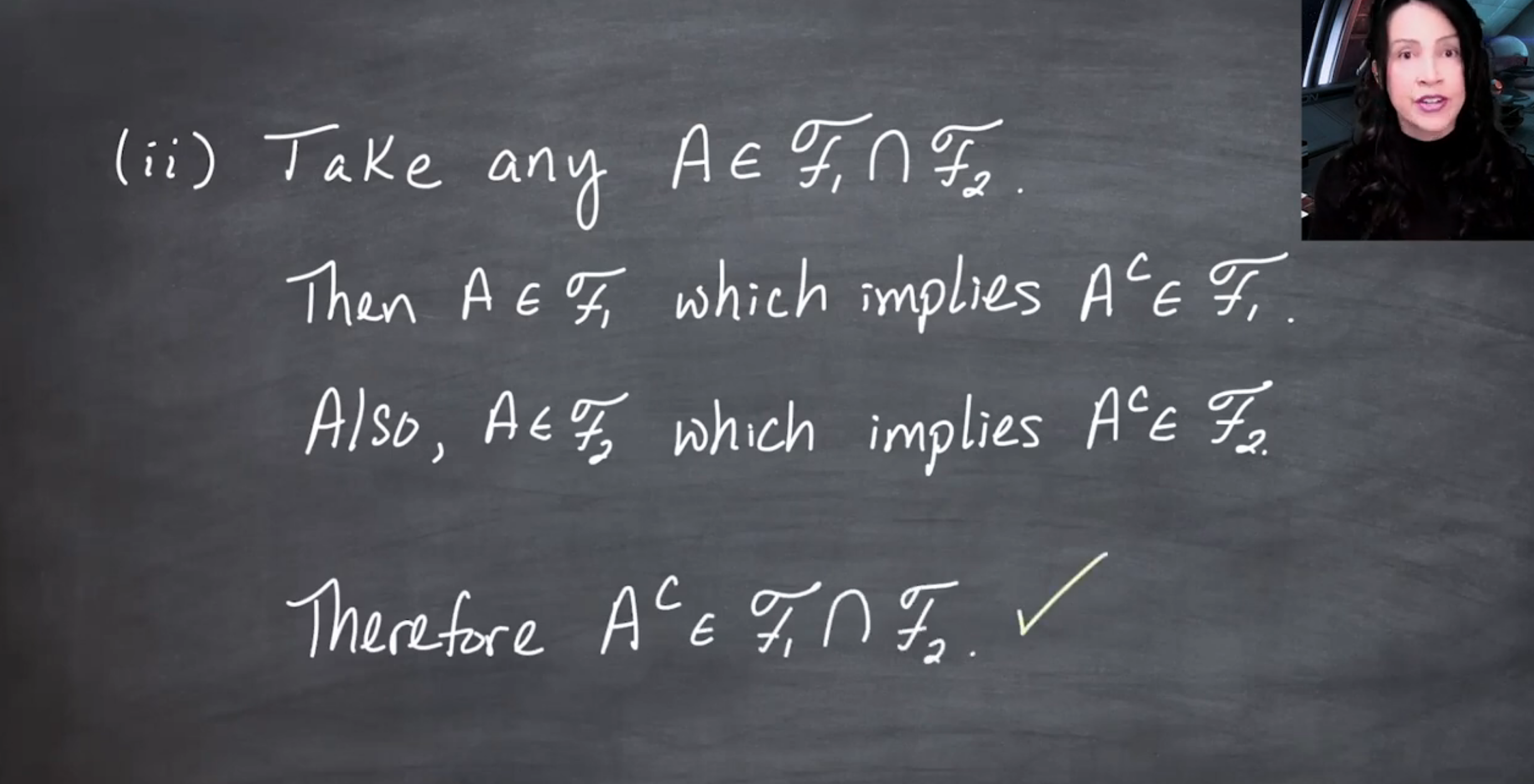
Second, take any set A \in \mathcal{F}_1 \cap \mathcal{F}_2. Then A \in \mathcal{F}_1 and A \in \mathcal{F}_2. Since each is a \sigma-field,
A^c \in \mathcal{F}_1 \quad \text{and} \quad A^c \in \mathcal{F}_2.
So
A^c \in \mathcal{F}_1 \cap \mathcal{F}_2.
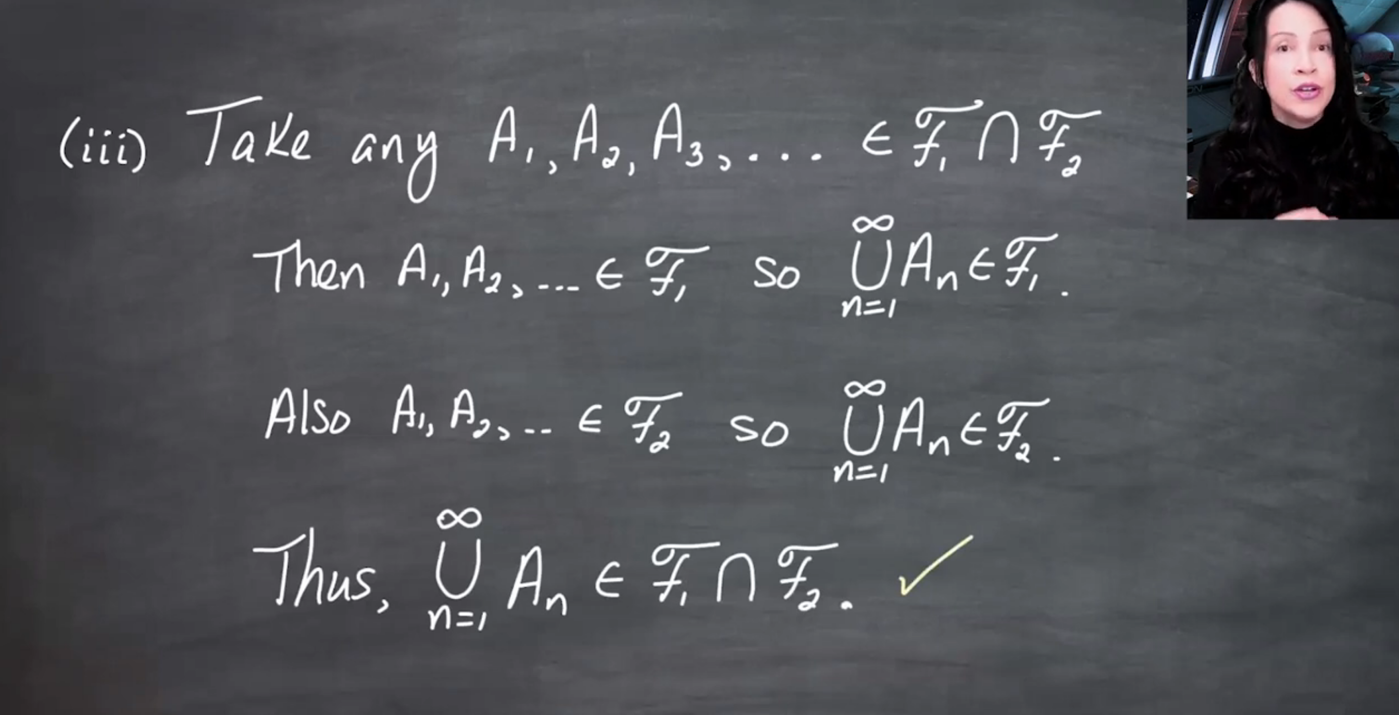
Third, take A_1,A_2,A_3,\ldots \in \mathcal{F}_1 \cap \mathcal{F}_2. Then every A_n belongs to both \mathcal{F}_1 and \mathcal{F}_2. Since each \sigma-field is closed under countable unions,
\bigcup_{n=1}^{\infty} A_n \in \mathcal{F}_1 \quad \text{and} \quad \bigcup_{n=1}^{\infty} A_n \in \mathcal{F}_2.
Therefore,
\bigcup_{n=1}^{\infty} A_n \in \mathcal{F}_1 \cap \mathcal{F}_2.
So \mathcal{F}_1 \cap \mathcal{F}_2 is a \sigma-field.
147.1.4 Monotonicity of generated \sigma-fields
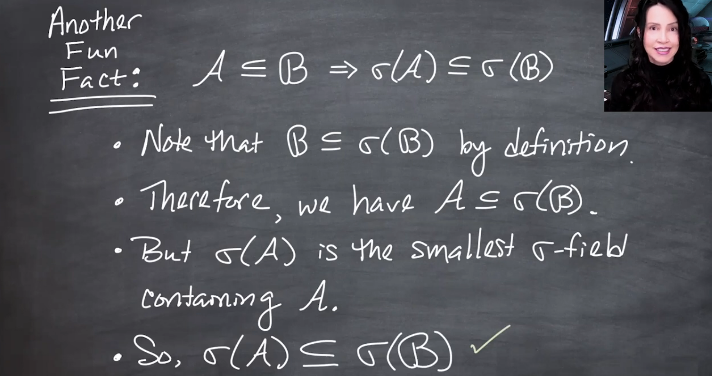
If
\mathcal{A} \subseteq \mathcal{B},
then
\sigma(\mathcal{A}) \subseteq \sigma(\mathcal{B}).
Reason: \mathcal{B} \subseteq \sigma(\mathcal{B}) by definition. Since \mathcal{A} \subseteq \mathcal{B}, we also have \mathcal{A} \subseteq \sigma(\mathcal{B}). But \sigma(\mathcal{A}) is the smallest \sigma-field containing \mathcal{A}, so it must be contained in \sigma(\mathcal{B}).
147.1.5 Simple examples
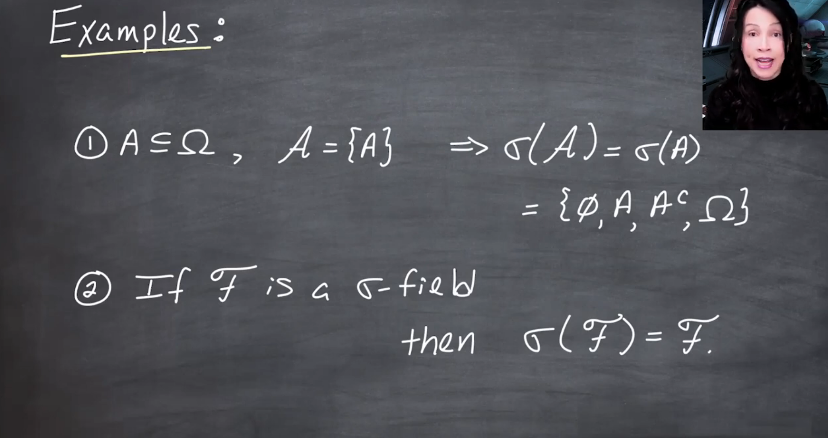
If \mathcal{A}=\{A\}, then
\sigma(\mathcal{A}) = \sigma(A) = \{\emptyset, A, A^c, \Omega\}.
If \mathcal{F} is already a \sigma-field, then
\sigma(\mathcal{F}) = \mathcal{F}.
Generating a \sigma-field from something already closed under the required operations adds nothing.
147.2 The Borel \sigma-field
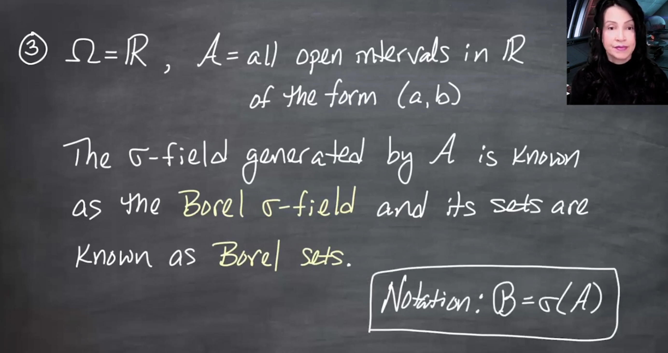
The important example is obtained by taking
\Omega = \mathbb{R}
and letting \mathcal{A} be the collection of all open intervals:
\mathcal{A} = \{(a,b): a,b \in \mathbb{R}, a < b\}.
Definition 147.2 (Borel \sigma-field on \mathbb{R}) The Borel \sigma-field on \mathbb{R} is
\mathcal{B}(\mathbb{R}) = \sigma\left(\{(a,b): a,b \in \mathbb{R}, a<b\}\right).
The sets in \mathcal{B}(\mathbb{R}) are called Borel sets.
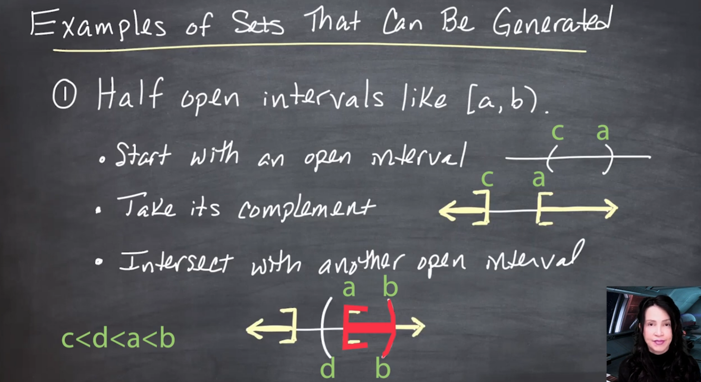
147.2.1 Examples of Borel sets
The Borel \sigma-field starts from open intervals, but it contains many other familiar subsets of \mathbb{R}.
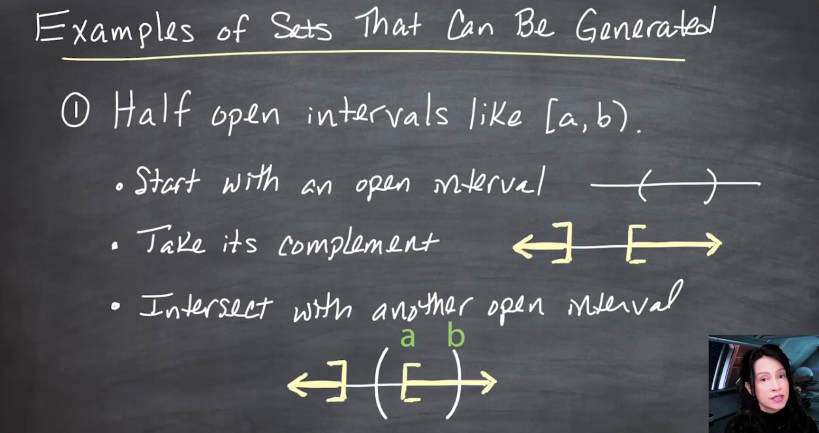
First, intervals of the form [a,b) are Borel. Choose numbers
c < d < a < b.
Then
[a,b) = (c,a)^c \cap (d,b).
The interval (c,a) is open, hence Borel; its complement is Borel; and (d,b) is open, hence Borel. Therefore their intersection is Borel.
The symmetric argument gives intervals of the form (a,b].
![Board note: similarly form (a,b] and then construct [a,b].](images/l02-s17.png)
Closed intervals are also Borel, since
[a,b] = [a,b) \cup (a,b].
A \sigma-field is closed under countable unions, and therefore also under finite unions.
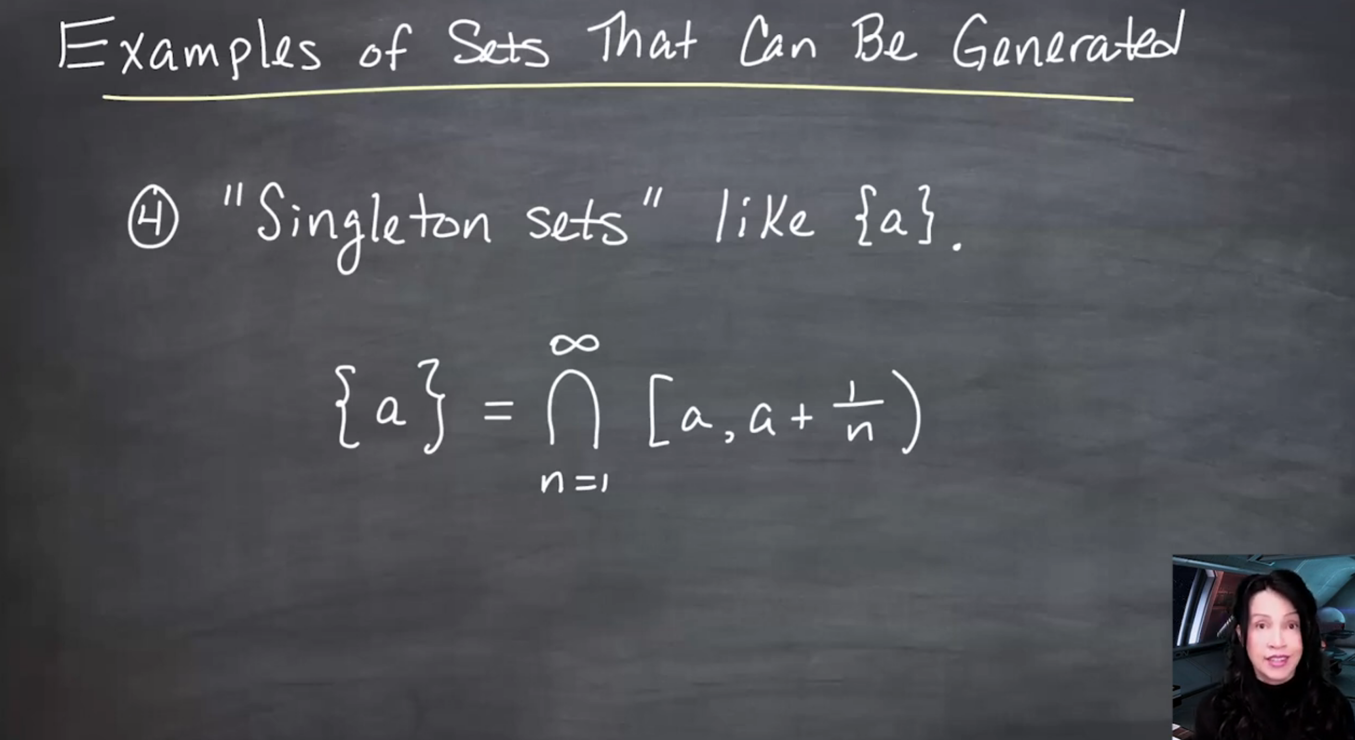
Singleton sets are Borel. One way to see this is
\{a\} = \bigcap_{n=1}^{\infty} \left[a, a + \frac{1}{n}\right).
Each interval on the right is Borel, and \sigma-fields are closed under countable intersections, so \{a\} is Borel.
Borel sets include many familiar sets, but not every subset of \mathbb{R} is Borel. Non-Borel subsets of \mathbb{R} require more advanced constructions and appear later.
147.3 Equivalent ways to generate \mathcal{B}(\mathbb{R})
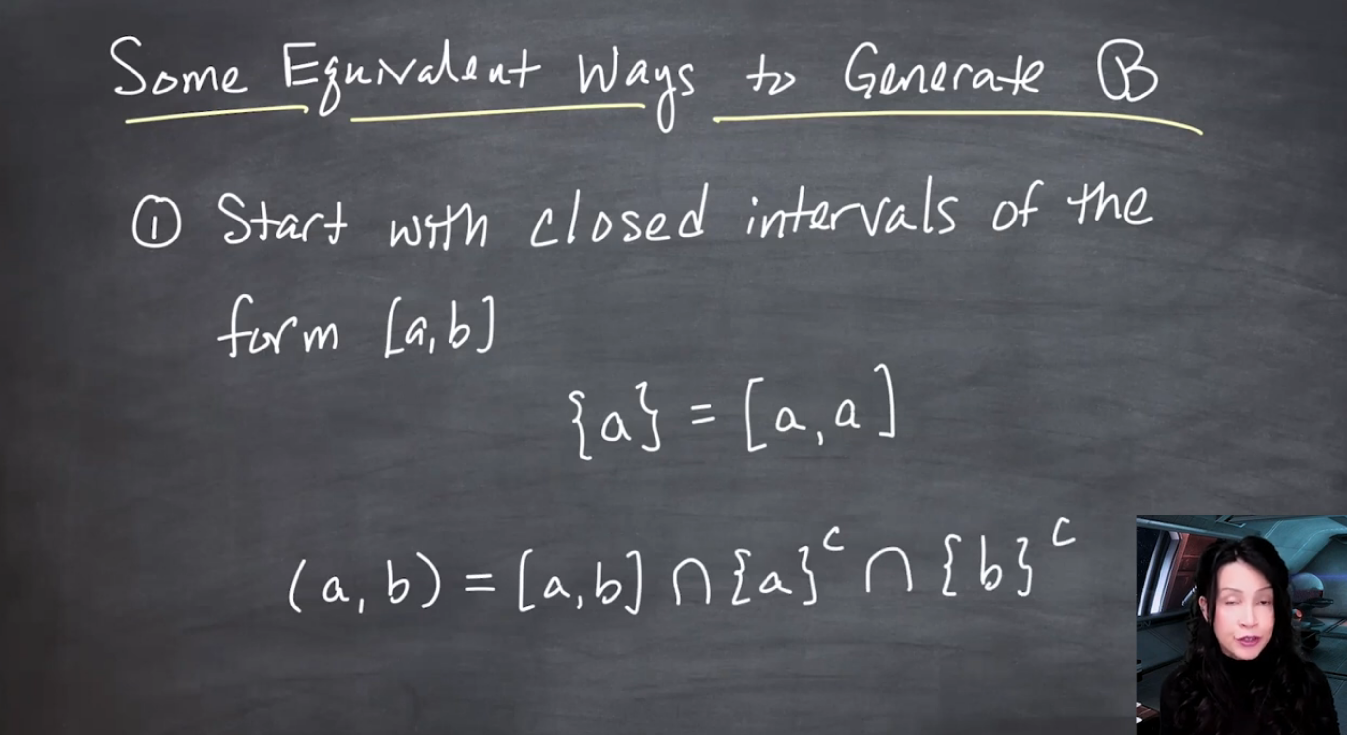
The Borel \sigma-field can also be generated from closed intervals:
\mathcal{B}(\mathbb{R}) = \sigma\left(\{[a,b]: a,b \in \mathbb{R}, a<b\}\right).
The reason is two-directional:
- Starting from open intervals, we already generated closed intervals.
- Starting from closed intervals, we can recover open intervals because
\{a\}=[a,a]
and therefore
(a,b) = [a,b] \cap \{a\}^c \cap \{b\}^c.
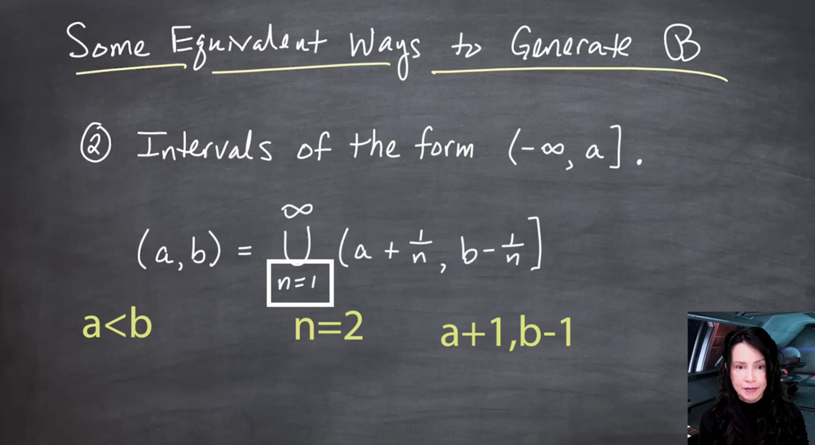
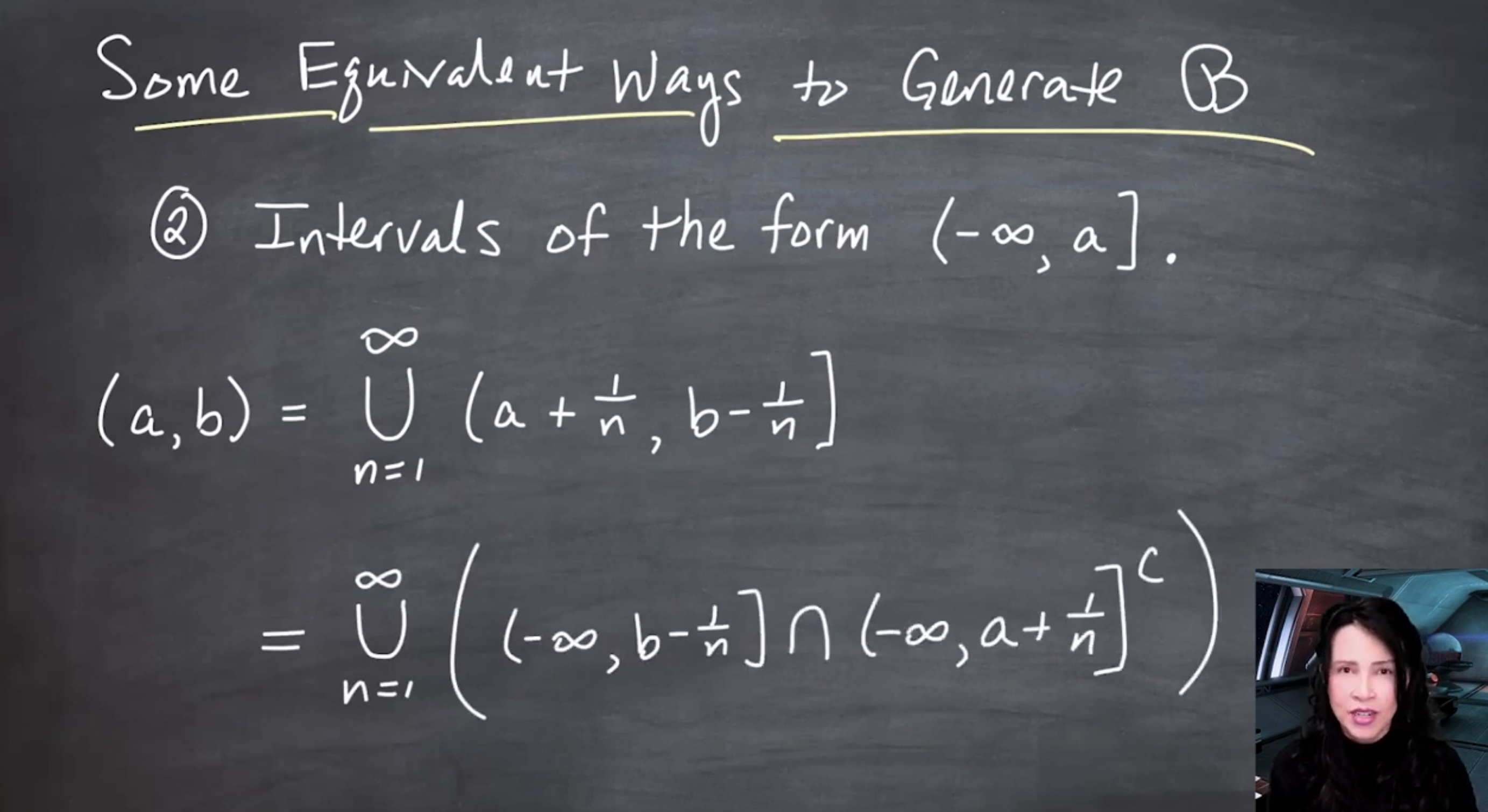
Another equivalent generator is the family of left-infinite closed rays:
\mathcal{B}(\mathbb{R}) = \sigma\left(\{(-\infty,a]: a \in \mathbb{R}\}\right).
To recover open intervals from these rays, first express
(a,b) = \bigcup_{n=N}^{\infty} \left(a+\frac{1}{n}, b-\frac{1}{n}\right]
where N is chosen large enough that a+\frac{1}{N}<b-\frac{1}{N}.
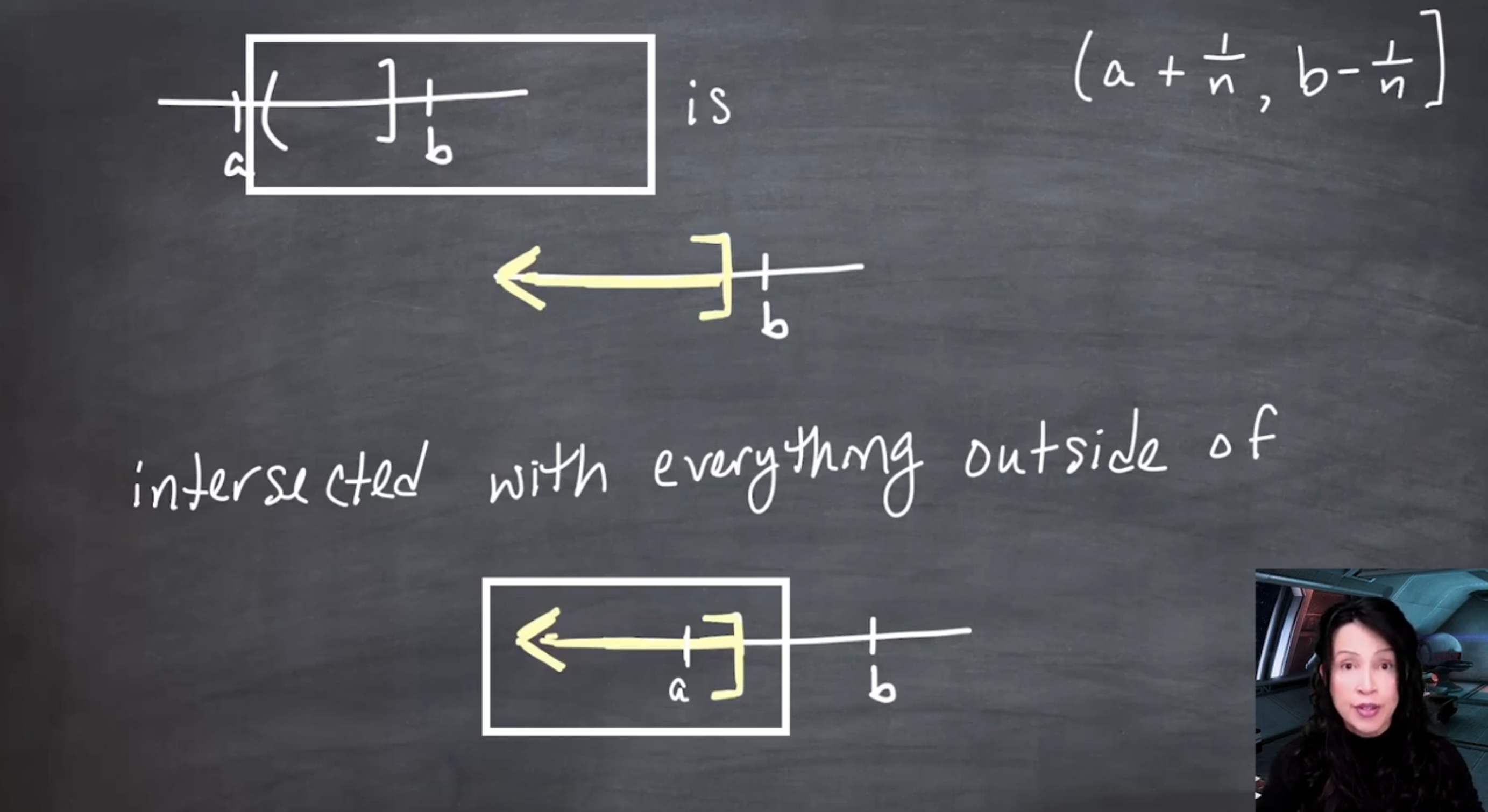
Each interval in the union can be written as
\left(a+\frac{1}{n}, b-\frac{1}{n}\right] = \left(-\infty, b-\frac{1}{n}\right] \cap \left(-\infty, a+\frac{1}{n}\right]^c.
So these intervals belong to the \sigma-field generated by the rays (-\infty,a], and the countable union gives (a,b).
A further fact, mentioned but not proved in the lesson, is that it is enough to use rational endpoints:
\mathcal{B}(\mathbb{R}) = \sigma\left(\{(-\infty,q]: q \in \mathbb{Q}\}\right).
This works because \mathbb{Q} is dense in \mathbb{R}: between any two real numbers there is a rational number.
147.3.1 Lesson summary
The structure of the lesson is:
\text{start with simple sets} \quad \longrightarrow \quad \text{generate a } \sigma\text{-field} \quad \longrightarrow \quad \text{define Borel sets on } \mathbb{R}.
The key idea is that a generated \sigma-field gives the minimal measurable universe forced by the sets we start with. For real-valued probability, the central measurable universe is the Borel \sigma-field \mathcal{B}(\mathbb{R}).