---
title: "Gibbs sampling - M2L5"
subtitle: "Bayesian Statistics: Techniques and Models"
description: "An introduction to the Gibbs sampling algorithm for sampling from complex probability distributions."
categories:
- Monte Carlo Estimation
keywords:
- Gibbs sampling
- Markov Chain Monte Carlo
- Full conditional distributions
- Bayesian inference
- MCMC
- Conditional distributions
- Conjugate priors
- Normal distribution
- Inverse gamma distribution
- Scaled inverse chi-square distribution
- R programming
- Statistical modeling
- Bayesian statistics
---
Gibbs sampling is a Gibbs sampling is named after the physicist Josiah Willard Gibbs, in reference to an analogy between the sampling algorithm and statistical physics. The algorithm was described in [@geman1984] by brothers *Stuart and Donald Geman*, and became popularized in the statistics community for calculating marginal probability distribution, especially the posterior distribution. Gibbs sampling is better suited for sampling from models with many variables by sampling them one at a time from a full conditional distribution.
::: { #fig-gibbs-sampler .column-margin group="slides" width="53mm"}

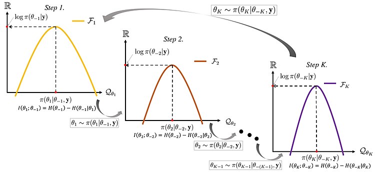
- Gibbs sampler cartoon:
- Each panel (Step 1, Step 2, …, Step K) showd the 1D conditional distribution for a single coordinate $(\theta_{k}\mid\theta_{-k},y)$
- The cartoon has a $log \pi(\theta_{-k}\mid y)$ as a reminder of "log posterior thinking."
- The red dot on the x-axis is the new sampled value for that co-ordinate
- The dashed vertical line indicates where we sampled x
- The dashed horizontal line indicates the corresponding value of the conditional distribution at the new sampled value
- The red dot on the y-axis is the value of the conditional distribution at the new sampled value
- $I(\cdot)$ is the information and $H(\cdot)$ is the entropy indicating a way to quantify how much knowing one block of variables reduces uncertainty about the other. This matters because in the Gibbs sampler, the chain often mixes slowly: updating one coordinate doesn't "forget" the others quickly because the posterior ties them together. So lower mutual information and higher entropy means faster mixing.
- The big arrow on top indicates the next step of the Gibbs sampler, which is to update the next sweep!
Statmath, CC BY-SA 4.0 <https://creativecommons.org/licenses/by-sa/4.0>, via Wikimedia Commons
:::
::: {.callout-tip}
### How does the Gibbs sampling simplify updating multiple parameters in MCMC?
It divides the process into updating one parameter at a time using (potentially convenient) full conditional distributions. The price we pay for this convenience is
1. the work required to find full conditional distributions and
2. the sampler may require more iterations to fully explore the posterior distribution as the draws tend to be more correlated since they share information in the form of parameters.
It is also possible to run a Gibbs sampler that draws from the "full" conditional distribution of multiple parameters. We would then cycle through and update blocks of parameters.
:::
### Multiple parameter sampling and full conditional distributions :movie_camera: {#sec-multiple-parameter-sampling}
{#fig-multiple-parameter-sampling .column-margin group="slides" width="53mm"}
So far, we have demonstrated MCMC for a single parameter.
What if we seek the posterior distribution of multiple parameters, and that posterior distribution does not have a standard form?
One option is to perform Metropolis-Hastings (M-H) by sampling candidates for all parameters at once, and accepting or rejecting all of those candidates together. While this is possible, it can get complicated.
Another (simpler) option is to sample the parameters one at a time.
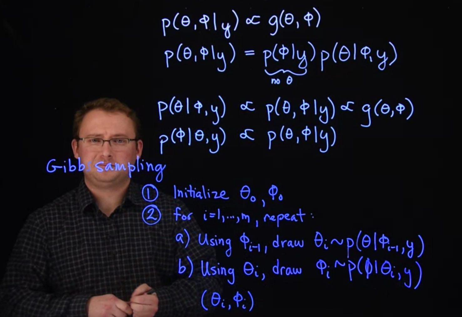
As a simple example, suppose we have a joint posterior distribution for two parameters $\theta$ and $\phi$, written $\mathbb{P}r(\theta, \phi \mid y) \propto g(\theta, \phi)$.
If we knew the value of $\phi$, then we would just draw a candidate for $\theta$ and use $g(\theta, \phi)$ to compute our Metropolis-Hastings ratio, and possibly accept the candidate.
Before moving on to the next iteration, if we don't know $\phi$, then we can perform a similar update for it.
Draw a candidate for $\phi$ using some proposal distribution and again use $g(\theta, \phi)$ to compute our Metropolis-Hastings ratio.
Here we pretend we know the value of $\theta$ by substituting its current iteration from the Markov chain.
Once we've drawn for both $\theta$ and $\phi$, that completes one iteration and we begin the next iteration by drawing a new $\theta$.
In other words, we're just going back and forth, updating the parameters one at a time, plugging the current value of the other parameter into $g(\theta, \phi)$.
This idea of one-at-a-time updates is used in what we call *Gibbs sampling*, which also produces a stationary Markov chain (whose stationary distribution is the posterior).
If you recall, this is the namesake of `JAGS`, "just another Gibbs sampler."
### Full conditional distributions
Before describing the full **Gibbs sampling algorithm** \index{Gibbs sampling algorithm}, there's one more thing we can do.
Using the chain rule of probability, we have
$$
\mathbb{P}r(\theta, \phi \mid y) = \mathbb{P}r(\theta \mid \phi, y) \cdot \mathbb{P}r(\phi \mid y)
$$
Notice that the only difference between $\mathbb{P}r(\theta, \phi \mid y)$ and $\mathbb{P}r(\theta \mid \phi, y)$ is multiplication by a factor that doesn't involve $\theta$. Since the $g(\theta, \phi)$ function above, when viewed as a function of $\theta$ is proportional to both these expressions, we might as well have replaced it with $\mathbb{P}r(\theta \mid \phi, y)$ in our update for $\theta$.
This distribution $\mathbb{P}r(\theta \mid \phi, y)$ is called the **full conditional distribution** [**Full conditional distribution**]{.column-margin} for $\theta$. \index{distribution!full conditional }
Why use $\mathbb{P}r(\theta \mid \phi, y)$ instead of $g(\theta, \phi)$?
In some cases, the full conditional distribution is a standard distribution we know how to sample. If that happens, we no longer need to draw a candidate and decide whether to accept it. In fact, if we treat the full conditional distribution as a candidate proposal distribution, the resulting Metropolis-Hastings acceptance probability becomes exactly 1.
Gibbs samplers require a little more work up front because you need to find the full conditional distribution for each parameter. The good news is that all full conditional distributions have the same starting point: the full joint posterior distribution. Using the example above, we have
$$
\mathbb{P}r(\theta \mid \phi, y) \propto \mathbb{P}r(\theta, \phi \mid y)
$$ {#eq-full-conditional-proportional-to-joint-posterior}
where we simply now treat $\phi$ as a known number. Likewise, the other full conditional is $\mathbb{P}r(\phi \mid \theta, y) \propto \mathbb{P}r(\theta, \phi \mid y)$ where here, we consider $\theta$ to be a known number. We always start with the full posterior distribution. Thus, the process of finding full conditional distributions is the same as finding the posterior distribution of each parameter, pretending that all other parameters are known.
### Gibbs sampler
Here is the algorithm.
::: {#alg-gibbs-sampler}
```pseudocode
#| html-indent-size: "1.2em"
#| html-comment-delimiter: "//"
#| html-line-number: true
#| html-line-number-punc: ":"
#| html-no-end: false
#| pdf-placement: "htb!"
#| pdf-line-number: true
#| pdf-comment-delimiter: "//"
\begin{algorithm}
\caption{Gibbs sampling algorithm for two parameters $\theta$ and $\phi$}
\begin{algorithmic}
\Procedure{GibbsSampler}{$\theta_0, \phi_0, m$}
\State Initialize $\theta_0, \phi_0$
\For{$i = 1$ \To $m$}
\State Draw a sample $\theta_i$ from $\mathbb{P}r(\theta \mid \phi = \phi_{i-1}, y)$
\State Draw a sample $\phi_i$ from $\mathbb{P}r(\phi \mid \theta = \theta_i, y)$
\EndFor
\EndProcedure
\end{algorithmic}
\end{algorithm}
```
:::
Here is a longer more verbose version of @alg-gibbs-sampler, which includes the case where there are more than two parameters.
<!-- convert this to refer to the above statement instead -->
Suppose we have a joint posterior distribution for two parameters $\theta$ and $\phi$, written $\mathbb{P}r(\theta, \phi \mid y)$. If we can find the distribution of each parameter at a time, i.e., $\mathbb{P}r(\theta \mid \phi, y)$ and $\mathbb{P}r(\phi \mid \theta, y)$, then we can take turns sampling these distributions like so:
1. Using $\phi_{i-1}$, draw $\theta_i$ from $\mathbb{P}r(\theta \mid \phi = \phi_{i-1}, y)$.
2. Using $\theta_i$, draw $\phi_i$ from $\mathbb{P}r(\phi \mid \theta = \theta_i, y)$.
Together, steps 1 and 2 complete one cycle of the Gibbs sampler and produce the draw for $(\theta_i, \phi_i)$ in one iteration of a MCMC sampler. If there are more than two parameters, we can handle that also. One Gibbs cycle would include an update for each of the parameters.
::: {.callout-tip}
## Gibbs sampler - TL--DR
The idea of @alg-gibbs-sampler is that we can **update multiple parameters by sampling just one parameter at a time**, cycling through all parameters and repeating.
To perform the update for one particular parameter, we substitute in the current values of the other parameters that we already sampled.
We must be **blessed** to be able to apply the divide and conquer strategy to the most horiffic looking posterior distribution, and find the full conditional distributions for each parameter. If we can do that, then we can sample from those full conditionals directly, and we don't need to worry about acceptance probabilities at all. The resulting Markov chain will have the correct stationary distribution, which is the full posterior distribution of all parameters.
:::
In the following segments, we will provide a concrete example of finding full conditional distributions and constructing a Gibbs sampler.
## Conditionally conjugate prior example with Normal likelihood :movie_camera: {#sec-conditionally-conjugate-prior-with-normal-likelihood}
### Normal likelihood, unknown mean and variance
{#fig-normal-likelihood-unknown-mean-and-variance .column-margin group="slides" width="53mm"}
{#fig-normal-likelihood-conjugate-prior .column-margin group="slides" width="53mm"}
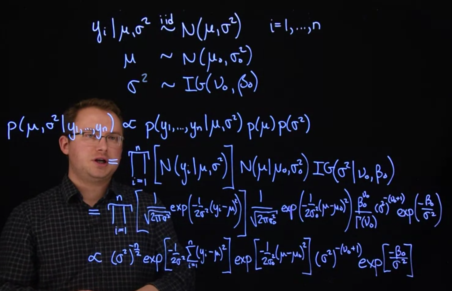
Let's return to the example at the end of Lesson 2 where we have normal likelihood with unknown mean and unknown variance. The model is:
$$
\begin{aligned}
y_i \mid \mu, \sigma^2 &\overset{\text{iid}}{\sim} \mathcal{N} ( \mu, \sigma^2 ), \quad i=1,\ldots,n \\
\mu &\sim \mathcal{N}(\mu_0, \sigma_0^2) \\
\sigma^2 &\sim \mathcal{IG}(\nu_0, \beta_0)
\end{aligned}
$$
We chose a normal prior for $\mu$ because, in the case where $\sigma^2$ is known, the normal is the conjugate prior for $\mu$. Likewise, in the case where $\mu$ is known, the inverse-gamma is the conjugate prior for $\sigma^2$. This will give us convenient full conditional distributions in a Gibbs sampler.
Let's first work out the form of the full posterior distribution. When we begin analyzing data, the `JAGS` software will complete this step for us. However, it is extremely valuable to see and understand how this works.
$$
\begin{aligned}
\mathbb{P}r( \mu, \sigma^2 \mid y_1, y_2, \ldots, y_n ) &\propto
\mathbb{P}r(y_1, y_2, \ldots, y_n \mid \mu, \sigma^2) \mathbb{P}r(\mu) \mathbb{P}r(\sigma^2)
\\ &= \prod_{i=1}^n \mathcal{N} ( y_i \mid \mu, \sigma^2 ) \times \mathcal{N}( \mu \mid \mu_0, \sigma_0^2) \times \mathcal{IG}(\sigma^2 \mid \nu_0, \beta_0)
\\ &= \prod_{i=1}^n \frac{1}{\sqrt{2\pi\sigma^2}}\exp \left[ -\frac{(y_i - \mu)^2}{2\sigma^2} \right]
\\ & \qquad \times\frac{1}{\sqrt{2\pi\sigma_0^2}} \exp \left[ -\frac{(\mu - \mu_0)^2}{2\sigma_0^2} \right]
\\ & \qquad \times \frac{\beta_0^{\nu_0}}{\Gamma(\nu_0)}(\sigma^2)^{-(\nu_0 + 1)} \exp \left[ -\frac{\beta_0}{\sigma^2} \right] \mathbb{I}_{\sigma^2 > 0}(\sigma^2)
\\ &\propto (\sigma^2)^{-n/2} \exp \left[ -\frac{\sum_{i=1}^n (y_i - \mu)^2}{2\sigma^2} \right]
\\ & \qquad \times \exp \left[ -\frac{(\mu - \mu_0)^2}{2\sigma_0^2} \right] (\sigma^2)^{-(\nu_0 + 1)}
\\ & \qquad \times \exp \left[ -\frac{\beta_0}{\sigma^2} \right] \mathbb{I}_{\sigma^2 > 0}(\sigma^2)
\end{aligned}
$$
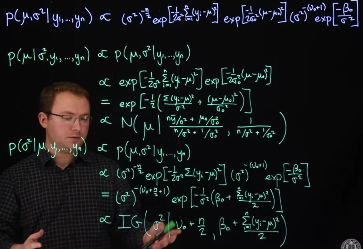
From here, it is easy to continue on to find the two full conditional distributions we need.
First let's look at $\mu$, assuming $\sigma^2$ is known (in which case it becomes a constant and is absorbed into the normalizing constant):
$$
\begin{aligned}
\mathbb{P}r(\mu \mid \sigma^2, y_1, \ldots, y_n) &\propto \mathbb{P}r( \mu, \sigma^2 \mid y_1, \ldots, y_n )
\\ &\propto \exp \left[ -\frac{\sum_{i=1}^n (y_i - \mu)^2}{2\sigma^2} \right] \exp \left[ -\frac{(\mu - \mu_0)^2}{2\sigma_0^2} \right]
\\ &\propto \exp \left[ -\frac{1}{2} \left( \frac{ \sum_{i=1}^n (y_i - \mu)^2}{2\sigma^2} + \frac{(\mu - \mu_0)^2}{2\sigma_0^2} \right) \right]
\\ &\propto \text{N} \left( \mu \mid \frac{n\bar{y}/\sigma^2 + \mu_0/\sigma_0^2}{n/\sigma^2 + 1/\sigma_0^2} \frac{1}{n/\sigma^2 + 1/\sigma_0^2} \right)
\end {aligned}
$$ {#eq-full-conditional-update-for-mean-derivation}
which we derived in the supplementary material of the last course. So, given the data and $\sigma^2$, $\mu$ follows this normal distribution.
Now let's look at $\sigma^2$, assuming $\mu$ is known:
$$
\begin{aligned}
\mathbb{P}r(\sigma^2 \mid \mu, y_1, \ldots, y_n) & \propto \mathbb{P}r( \mu, \sigma^2 \mid y_1, \ldots, y_n )
\\ &\propto (\sigma^2)^{-n/2} \exp \left[ -\frac{\sum_{i=1}^n (y_i - \mu)^2}{2\sigma^2} \right] (\sigma^2)^{-(\nu_0 + 1)} \exp \left[ -\frac{\beta_0}{\sigma^2} \right] I_{\sigma^2 > 0}(\sigma^2)
\\ &\propto (\sigma^2)^{-(\nu_0 + n/2 + 1)} \exp \left[ -\frac{1}{\sigma^2} \left( \beta_0 + \frac{\sum_{i=1}^n (y_i - \mu)^2}{2} \right) \right] I_{\sigma^2 > 0}(\sigma^2)
\\ &\propto \text{IG}\left( \sigma^2 \mid \nu_0 + \frac{n}{2}, \, \beta_0 + \frac{\sum_{i=1}^n (y_i - \mu)^2}{2} \right)
\end{aligned}
$$ {#eq-full-conditional-update-for-variance-derivation}
These two distributions provide the basis of a Gibbs sampler to simulate from a Markov chain whose stationary distribution is the full posterior of both $\mu$ and $\sigma^2$. We simply alternate draws between these two parameters, using the most recent draw of one parameter to update the other.
We will do this in `R` in the next segment.
## Computing example with Normal likelihood
To implement the Gibbs sampler we just described, let's return to our running example where the data are the percent change in total personnel from last year to this year for $n=10$ companies. [**Company personnel**]{.column-margin} We'll still use a **normal likelihood**, but now we'll *relax the assumption that we know the variance of growth between companies*, $\sigma^2$, and estimate that variance. Instead of the $t$ prior from earlier, we will use the **conditionally conjugate priors**, normal for $\mu$ and inverse-gamma for $\sigma^2$.
The first step will be to write functions to simulate from the full conditional distributions we derived in the previous segment. The full conditional for $\mu$, given $\sigma^2$ and data is
### Conditionally conjugate priors for the mean :movie_camera: {#sec-conditionally-conjugate-priors-for-mean}
$$
\text{N} \left( \mu \mid \frac{n\bar{y}/\sigma^2 + \mu_0/\sigma_0^2}{n/\sigma^2 + 1/\sigma_0^2}, \, \frac{1}{n/\sigma^2 + 1/\sigma_0^2} \right)
$$ {#eq-full-conditional-update-for-mean}
```{r}
#| label: C2-L05-1
#' update_mu
#'
#' @param n - sample size
#' @param ybar - sample mean
#' @param sig2 - current sigma squared
#' @param mu_0 - mean hyper-parameter
#' @param sig2_0 - variance hyper-parameter
#'
#' @output - updated value for mu the mean
update_mu = function(n, ybar, sig2, mu_0, sig2_0) { # <1>
sig2_1 = 1.0 / (n / sig2 + 1.0 / sig2_0) # <2>
mu_1 = sig2_1 * (n * ybar / sig2 + mu_0 / sig2_0) # <3>
rnorm(n=1, mean=mu_1, sd=sqrt(sig2_1)) # <4>
}
```
1. we don't need the data `y`
2. where: <br> `sig2_1` is $\sigma^2_1$ the right term in @eq-full-conditional-update-for-mean <br> `sig2` is the current $\sigma_2$ which we update in `update_sigma` below using @eq-full-conditional-update-for-variance <br> `sig2_0` is the hyper parameter for $\sigma^2_0$
3. `mu_1` is $\sigma^2_1$ the left term in @eq-full-conditional-update-for-mean which uses `sig2_1` we just computed
4. we now draw from the a $N(\mu_1,\sigma_1^2)$ for `update_sig2` and the `trace`.
### Conditionally conjugate priors for the variance
The full conditional for $\sigma^2$ given $\mu$ and data is
$$
\text{IG}\left( \sigma^2 \mid \nu_0 + \frac{n}{2}, \, \beta_0 + \frac{\sum_{i=1}^n (y_i - \mu)^2}{2} \right)
$$ {#eq-full-conditional-update-for-variance}
```{r}
#| label: C2-L05-2
#' update_sig2
#'
#' @param n - sample size
#' @param y - the data
#' @param nu_0 - nu hyper-parameter
#' @param beta_0 - beta hyper-parameter
#'
#' @output - updated value for sigma2 the variance
update_sig2 = function(n, y, mu, nu_0, beta_0) { # <1>
nu_1 = nu_0 + n / 2.0 # <2>
sumsq = sum( (y - mu)^2 ) # <3>
beta_1 = beta_0 + sumsq / 2.0 # <4>
out_gamma = rgamma(n=1, shape=nu_1, rate=beta_1) # <5>
1.0 / out_gamma # <6>
}
```
1. we need the data to update beta
2. `nu_1` the left term in @eq-full-conditional-update-for-variance
3. vectorized
4. `beta_1` the right term in @eq-full-conditional-update-for-variance
5. draw a gamma sample with updated `rate` for $\text{Gamma}()$ is `shape` for $\text{IG}()$ inv-gamma
6. since there is no `rinvgamma` in `R` we use the reciprocal of a gamma random variable which is distributed inv-gamma
With functions for drawing from the full conditionals, we are ready to write a function to perform Gibbs sampling.
### Gibbs sampler in `R`
```{r}
#| label: C2-L05-3
gibbs = function(y, n_iter, init, prior) {
ybar = mean(y)
n = length(y)
## initialize
mu_out = numeric(n_iter)
sig2_out = numeric(n_iter)
mu_now = init$mu
## Gibbs sampler
for (i in 1:n_iter) {
sig2_now = update_sig2(n=n, y=y, mu=mu_now, nu_0=prior$nu_0, beta_0=prior$beta_0)
mu_now = update_mu(n=n, ybar=ybar, sig2=sig2_now, mu_0=prior$mu_0, sig2_0=prior$sig2_0)
sig2_out[i] = sig2_now
mu_out[i] = mu_now
}
cbind(mu=mu_out, sig2=sig2_out) # <1>
}
```
1. `cbind` for column bind will take a lists of list and convert them into a matrix of collumns.
Now we are ready to set up the problem in `R`.
$$
\begin{aligned}
y_i \mid \mu, \sigma &\stackrel {iid} \sim \mathcal{N}(\mu,\sigma^2), \quad i=1,\ldots,n
\\ \mu &\sim \mathcal{N}(\mu_0,\sigma^2_0)
\\ \sigma^2 & \sim \mathcal{IG}(\nu,\beta_0)
\end{aligned}
$$ {#eq-gibbs-sampler-model-summary}
\index{MCMC!effective sample size}
We also need to create the prior hyperparameters for $\sigma^2$, $\nu_0$ and $\beta_0$. If we chose these hyperperameters carefully, they are interpretable as a prior guess for sigma squared, as well as a prior effective sample size to go with that guess.
The prior effective sample size. Which we'll call $n_0$, is two times this $\nu_0$ parameter. So in other words, the nu parameter will be the prior sample size Divided by 2. We're also going to create an initial guess for sigma squared, let's call it $s^2_0$. The relationship between $\beta_0$ and these two numbers is the following: It is the prior sample size times the prior guess divided by 2.
This particular parameterization of the *Inverse gamma* distribution is called the **Scaled Inverse Chi Square Distribution**, where the two parameters are $n_0$ and $s^2_0$.
```{r}
#| label: C2-L05-4
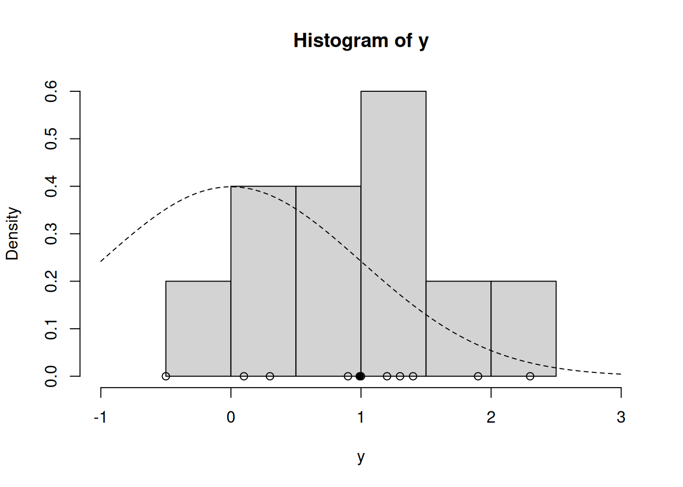
y = c(1.2, 1.4, -0.5, 0.3, 0.9, 2.3, 1.0, 0.1, 1.3, 1.9) # <1>
ybar = mean(y)
n = length(y)
## prior
prior = list()
prior$mu_0 = 0.0
prior$sig2_0 = 1.0
prior$n_0 = 2.0 # prior effective sample size for sig2
prior$s2_0 = 1.0 # prior point estimate for sig2
prior$nu_0 = prior$n_0 / 2.0 # prior parameter for inverse-gamma
prior$beta_0 = prior$n_0 * prior$s2_0 / 2.0 # prior parameter for inverse-gamma
hist(y, freq=FALSE, xlim=c(-1.0, 3.0)) # histogram of the data
curve(dnorm(x=x, mean = prior$mu_0, sd=sqrt(prior$sig2_0)), lty=2, add=TRUE) # prior for mu
points(y, rep(0,n), pch=1) # individual data points
points(ybar, 0, pch=19) # sample mean
```
Finally, we can initialize and run the sampler!
```{r}
#| label: C2-L05-5
set.seed(53)

init = list()
init$mu = 0.0

post = gibbs(y=y, n_iter=1e3, init=init, prior=prior)
```
```{r}
#| label: C2-L05-6
head(post)
```
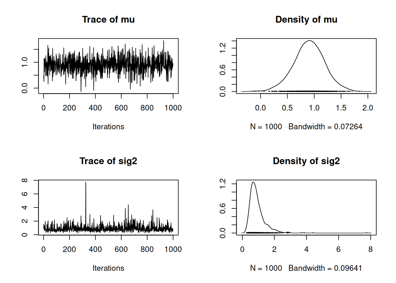
```{r}
#| label: C2-L05-7
library("coda")
plot(as.mcmc(post))
```
```{r}
#| label: C2-L05-8
summary(as.mcmc(post))
```
As with the Metropolis-Hastings example, these chains appear to have converged. In the next lesson, we will discuss convergence in greater detail.