142 1.4.3: How do I implement the Kalman-filter steps in Octave?

142.1 Introduction to lesson

• In this lesson, you will learn how to implement KF in Octave.
  
• It is recommended that you keep the KF equations nearby.

TipPrediction

Step 1a: State prediction (time update)

\hat{x}_k^- = A_{k-1}\hat{x}_{k-1}^+ + B_{k-1}u_{k-1}

Step 1b: Prediction-error covariance update

\Sigma_{\tilde{x},k}^- = A_{k-1}\Sigma_{x,k-1}^+ A_{k-1}^T + \Sigma_{\tilde{w}}

Step 1c: Predict system output

\hat{z}_k = C_k \hat{x}_k^- + D_k u_k

TipCorrection

Step 2a: Estimator gain matrix

L_k = \Sigma_{\tilde{x},k}^- C_k^T \left[C_k \Sigma_{\tilde{x},k}^- C_k^T + \Sigma_{\tilde{v}}\right]^{-1}

Step 2b: State estimate (measurement update)

\hat{x}_k^+ = \hat{x}_k^- + L_k (z_k - \hat{z}_k)

Step 2c: Estimation-error covariance update

\Sigma_{\tilde{x},k}^+ = (I - L_k C_k)\Sigma_{\tilde{x},k}^-

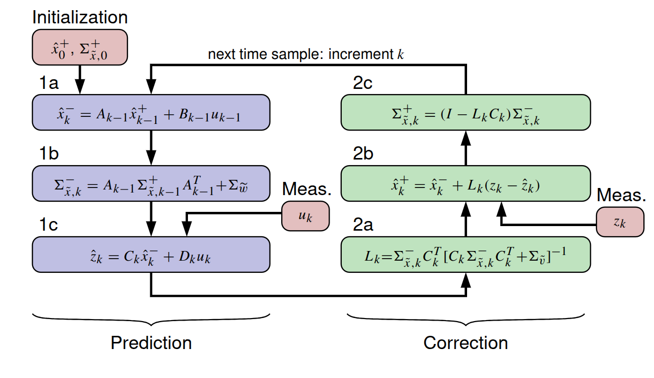
142.2 Visualizing the Linear Kalman Filter

• Linear Kalman-filter equations naturally form a recursion:
  • Initialization → Prediction → Correction → Next timestep
• Notes:
  • “Simple” to implement on a digital computer
    
  • Only six lines of code execute each iteration
    
  • Most effort is in setup and plotting

Figure 142.1: kf recursion

142.3 KF Step 1 (Prediction)

% Load data from simulation of system dynamic model
load simOut.mat Ad Bd Cd Dd SigmaV SigmaW dT t u x z

% Determine number of states and timesteps
[nx,nt] = size(x);

% Initialize state estimate and covariance
xhat = zeros(nx,1); 
SigmaX = zeros(nx,nx);

% Initialize storage for state/bounds for plotting purposes
xhatstore = zeros(nx,nt); 
boundstore = zeros(nx,nt);

for k = 2:length(t)

  % KF Step 1a: State prediction time update
  xhat = Ad*xhat + Bd*u(:,k-1); % use prior value of "u"

  % KF Step 1b: Prediction-error covariance time update
  SigmaX = Ad*SigmaX*Ad' + SigmaW;

  % KF Step 1c: Predict system output
  zhat = Cd*xhat + Dd*u(:,k); % use present value of "u"

142.4 KF Step 2 (Correction)

  % KF Step 2a: Compute estimator matrix
  L = SigmaX*Cd'/(Cd*SigmaX*Cd' + SigmaV);

  % KF Step 2b: State estimate measurement update
  xhat = xhat + L*(z(:,k) - zhat);

  % KF Step 2c: Estimation-error covariance measurement update
  SigmaX = (eye(nx) - L*Cd)*SigmaX;

  % Store estimate and bounds for evaluation / plotting purposes
  xhatstore(:,k) = xhat;
  boundstore(:,k) = 3*sqrt(diag(SigmaX));

end

• That’s it! We’re now ready to plot results.

142.5 Plot Results from KF Execution

figure(1); clf; % Plot the states and estimates

t2 = [t fliplr(t)]; % Prepare for plotting bounds via "fill"
x2 = [xhatstore - boundstore fliplr(xhatstore + boundstore)];

h1 = fill(t2,x2,'b','FaceAlpha',0.5,'LineStyle','none'); 
hold on; grid on

h2 = plot(t,x',t,xhatstore','--'); % Plot true state and estimate

legend([h2;h1], ...
  'True position','True velocity','Position estimate', ...
  'Velocity estimate','Bounds');

title('Demonstration of Kalman filter state estimates');
xlabel('Time (s)'); 
ylabel('State (m or m/s)');

figure(2); clf;

xerr = x - xhatstore; % Plot state-estimation errors

for k = 1:nx
  subplot(nx,1,k);

  fill(t2,[-boundstore(k,:) fliplr(boundstore(k,:))],'b', ...
       'FaceAlpha',0.25,'LineStyle','none'); 
  hold on; grid on;

  plot(t,xerr(k,:),'b');

  title(sprintf('State %d estimation error with bounds',k));
  xlabel('Time (s)'); 
  ylabel('Error');
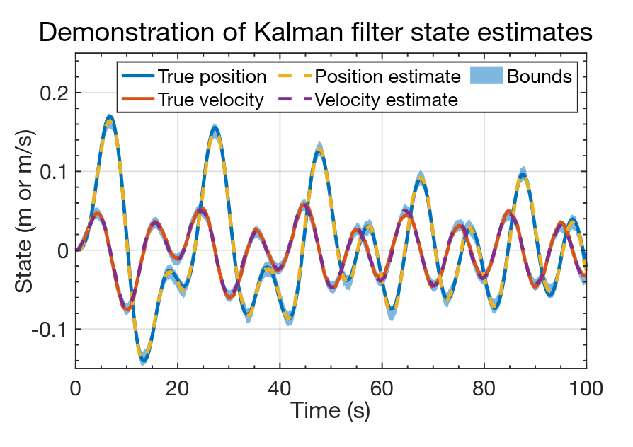
end

142.6 Sample Results: States and Estimates

• Output shown for spring-mass-damper example using simulation data.
• True states and estimated states are plotted with confidence bounds.

Key observations:

• KF estimates both position and velocity well
• Errors do not converge to zero
• Estimates remain within confidence bounds (as expected)

Figure 142.2: Demonstration of Kalman filter state estimates

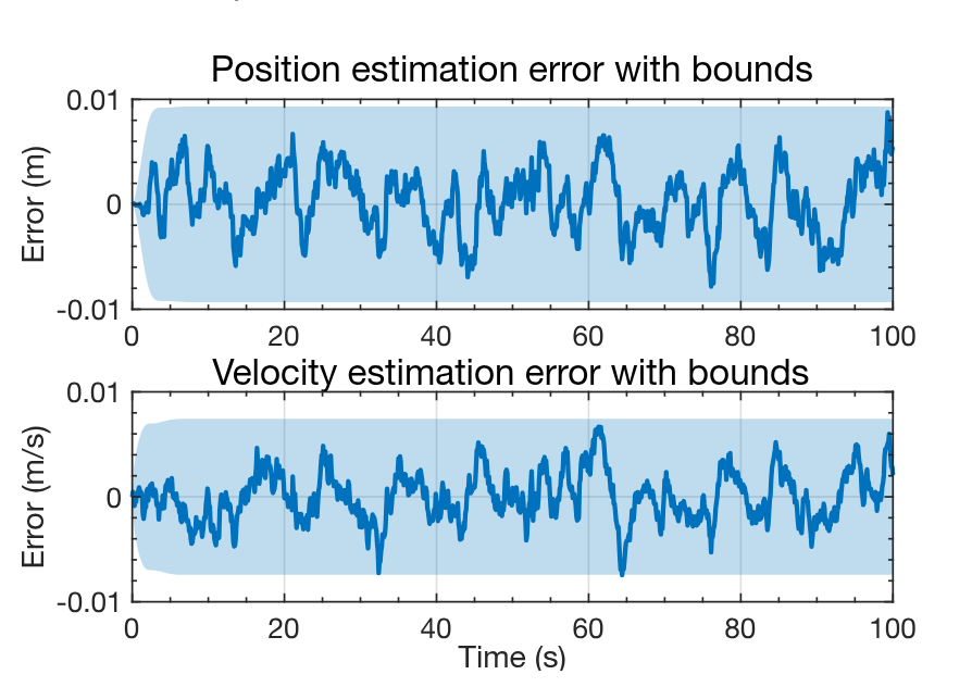
142.7 Sample Results: Estimation Errors

• Alternative visualization: plot estimation errors directly

Insights:

• Errors always contain a random component (due to process noise (w_k))
• Easier to verify confidence bounds

Observations:

• Position estimate remains within bounds
• Velocity estimate exceeds bounds once (≈ 0.1% of time)
• Matches theoretical expectation (~99.7% confidence bounds)

Figure 142.3: Estimation error with bounds

142.8 Summary

You have learned how to:

• Implement KF steps in Octave code
• Plot KF output in two ways

Notes:

• Code is general (not system-specific)
• Applies to any linear system satisfying KF assumptions
• Results provide intuition for KF behavior