128.1 Converting continuous-time state-space models to discrete-time
Here are question to consider as we learn how to convert continuous-time state-space models to discrete-time state-space models:
- What is the difference between continuous-time and discrete-time state-space models?
- which matrix are the same for continuous-time and discrete-time state-space models?
- for the rest how do we convert continuous-time state-space models to discrete-time state-space models?
- any shortcuts to remember?
128.1.1 Discrete-time state-space models
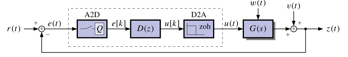
- Computer monitoring of real-time systems requires analog-to-digital (A2D) and digital-to-analog (D2A) conversion
- Linear discrete-time systems can also be represented in state-space form:
\begin{aligned} x_{t+1} &= A_dx_t + B_du_t + w_t && \text{state eqn.}\\ z_t &= C_dx_t + D_du_t + v_t && \text{observation eqn.} \end{aligned} \tag{128.1}
- The subscript d emphasizes that, in general, the A, B, C and D matrices are different for the same discrete-time and continuous-time system.
- The d subscript will usually be dropped as it can be interpreted from the context.
128.1.2 Time (dynamic) response of discrete-time models
The full solution, via induction from x_{t+1} = A_d x_t + B_d u_t + w_t, is:
x_{t} = A_d^t x_0 + \underbrace{\sum_{j=0}^{t-1} A_d^{t-j-1} B_d u_j }_{\text{convolution}} \tag{128.2}
Since z_t = C_d x_t + D_d u_t, we also have:
z_t= \underbrace{C_d A_d^t x_0}_{\text{initial response}}+ \underbrace{\sum_{j=0}^{t-1} C_d A_d^{t-j-1} B_d u_j }_{\text{convolution}} \underbrace{+ D_d u_t}_{\text{feed-through}} \tag{128.3}
- Comparing with the continuous-time solution,
- e^{At} has been replaced by A_d^t and
- integrals have been replaced by summations
Note: we wont cover the proof by induction and these are covered in Linear Systems Theory.
128.1.3 Converting plant dynamics to discrete time (1)
- Combine the dynamics of the zero-order hold and the plant.
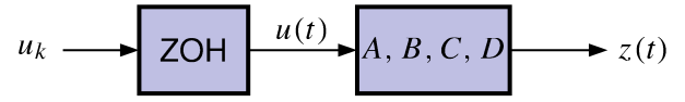
Recall that the continuous-time state dynamics of the plant are: \dot{x} = Ax(t) + Bu(t)
Evaluate x(t) at discrete times. Recall also the solution for x(t):
x(t) = \int_0^t e^{A(t-\tau)} B u(\tau) d\tau
x_{t+1}(t) = x((t+1)\Delta t) = \int_0^{(t+1)\Delta t} e^{A((t+1)\Delta t-\tau)} B u(\tau) d\tau
128.1.4 Converting plant dynamics to discrete time (2)
- We break up the integral into two pieces:
\begin{aligned} x_{k+1}(t) &= \int_0^{k\Delta t} e^{A((k+1)\Delta t-\tau)} B u(\tau) d\tau \\ &= \int_0^{k\Delta t} e^{A((k+1)\Delta t-\tau)} B u(\tau) d\tau + \int_{k\Delta t}^{(k+1)\Delta t} e^{A((k+1)\Delta t-\tau)} B u(\tau) d\tau \\ &= \int_0^{k\Delta t} e^{A\Delta t}e^{A((k)\Delta t-\tau)} B u(\tau) d\tau + \int_{k\Delta t}^{(k+1)\Delta t} e^{A((k+1)\Delta t-\tau)} B u(\tau) d\tau \\ &= e^{A\Delta t}x(k\Delta t) + \int_{k\Delta t}^{(k+1)\Delta t} e^{A((k+1)\Delta t-\tau)} B u(\tau) d\tau \end{aligned}
The first integral has become A_d \times x(k \Delta t) The second will become B_d \times u(k \Delta t) after a little more work
128.1.5 Converting plant dynamics to discrete time (3)
- In the remaining integral, note that u(\tau) is assumed to be constant from k\Delta t to (k+1)\Delta t; and equal to u(k\Delta t).
- We evaluate the integral via change of variables.
- Let \sigma = (k+1)\Delta t - \tau,
- \tau = (k+1)\Delta t - \sigma, and
- d\tau = -d\sigma.
\begin{aligned} x_{k+1} & = e^{A\Delta t}x(k\Delta t) + \int_{k\Delta t}^{(k+1)\Delta t} e^{A((k+1)\Delta t-\tau)} B u(\tau)\; d\tau \\ &= e^{A\Delta t}x(k\Delta t) + \left [\int_{(k+1)\Delta t}^{\Delta t} e^{A\sigma} B\; d\sigma \right ] u(k\Delta t)\\ &= \underbrace{ e^{A\Delta t}}_{A_d}\; x_k + \underbrace{ \left [\int_{(k+1)\Delta t}^{\Delta t} e^{A\sigma} B\; d\sigma \right ] u_k }_{B_d} \end{aligned}
128.1.6 Computing A_d, C_d, and D_d
Summarizing to this point, we have a discrete-time state-space representation from the continuous-time representation: x_{k+1} = A_d x_k + B_d u_k
where
- A_d = e^{A\Delta t} and
- B_d = \int_0^{\Delta t} e^{A(\Delta t-\sigma)} B d\sigma.
Similarly, we have: z_k = C_d x_k + D_d u_k.
where
- C_d = C and
- D_d = D.
There is no conversion for the C and D matrices,
The conversion for A is straightforward via the matrix exponential A_d = e^{A\Delta t}.
If Octave, we can type in:
Ad = expm(A*dT).Otherwise, we’ll need to compute e^{A\Delta t} = \mathcal{L}^{-1}\left[(sI - A)^{-1}\right]\Big|_{t = \Delta t}
128.1.7 Computing B_d
Now we focus on computing B_d . Recall that: \begin{aligned} B_d &= \int_0^{\Delta_t} e^{A(\Delta_t-\sigma)} B d\sigma \\ &= \int_0^{\Delta_t} \left( I + A(\sigma) + \frac{1}{2!}A^2(\sigma)^2 + \cdots \right) B d\sigma \\ &= \int_0^{\Delta_t} \left( I + \Delta t + \frac{1}{2!}(\Delta t)^2 + \cdots \right) B d\sigma \\ &= \left( I + \Delta t + \frac{1}{2!}(\Delta t)^2 + A^2 \frac{1}{2!}(\Delta t)^3 + \cdots \right) B \\ &= A^{-1}(e^{A\Delta_t} - I)B \\ &= A^{-1}(A_d - I)B. \end{aligned}
If A is invertible, this method works nicely!
Otherwise, we will need to perform the integral in the first line manually.
Also, in Octave,
[Ad,Bd]=c2d(A,B,dT)
128.1.8 Summary
- Computer monitoring of physical systems requires A2D and D2A conversion.
- The system that is “seen” by the computer is a discrete-time system, and must be represented by a discrete-time state-space model:
\begin{aligned} x_{t+1} &= A_dx_t + B_du_t + w_t && \text{state eqn.}\\ z_t &= C_dx_t + D_du_t + v_t && \text{observation eqn.} \end{aligned}
- Generally, the discrete A, B, C and D matrices differ from their continuous-time counterparts.
- We have learned to convert from the continuous A, B, C and D matrices to the discrete-time A_d, B_d, C_d and D_d matrices.
- Next we will see some examples of converting continuous-time to discrete-time and of simulating discrete-time state-space models.