---
title: "Lesson 1.2.2: The Target Tracking application"
subtitle: "Kalman Filter Boot Camp (and State Estimation)"
description: "This lesson introduces the Target Tracking application, a common use case for Kalman Filters, and explores different models for tracking a target's position over time."
categories:
- "Probability and Statistics"
- "Target tracking"
keywords:
- "Kalman Filter"
- "state estimation"
- "linear algebra"
---
## The Target Tracking application {#sec-kf-1.2.2-target-tracking}
::: {.callout-tip collapse="true"}
### Greek Notation
1. This section uses Greek letters to denote motion in the x and y direction.
2. The state vector is defined as $x(t) = [\xi(t), \eta(t), \dot{\xi}(t), \dot{\eta}(t)]^T$.
3. The reason is rather mundane - the instructor avoids circular definitions and any chance of confusion arising from reusing the same letter for different things. $X$ is already taken for the state vector. So we use $\xi$ and $\eta$ for the $x$ and $y$ coordinates, respectively.
4. He also uses $k$ for time index which I have replaced.
:::
- One application of KFs is for target tracking. [**target tracking problem**]{.column-margin}
- We wish to predict the future location of a dynamic system (the target) based on KF estimates and measurements.
- Ideally we know all the matrices and signals of its continuous-time linear state-space model
$$
\begin{aligned}
\dot{x}_t &= A x(t) + B u(t) + w(t) \\
z_t &= C x(t) + D u(t) + v(t)
\end{aligned}
$$ {#eq-target-tracking-equations}
- in The Target Tracking application, we typically don't know u(t)$ nor the state space matrices very well.
- we may need to approximate target dynamics based on some assumed behaviors.
- One idea is to come up with a hyper-prior that allows us to assign *intuitive* dynamics to the target. c.f. [@battagliaintuitive] work on intuitive physics
- If we roll our own we might use:
- a nearly constant position (NCP) model,
- a near constant velocity (NCV) model, or
- a coordinated-turn (CT) model.
- A quick search reveals that there are a few additional models like:
- a constant acceleration (CA) model,
- a constant jerk (CJ) model,
- a Singer model, and
- Stop-and-go (SAG) model, which is a special case of the Singer model.
- a random-maneuvering model.
- IMM - this is a regime-switching model that allows the target to switch between different motion models (e.g., NCP, NCV, CT) based on certain probabilities. It is particularly useful for tracking targets that exhibit varying motion patterns. IMM is due to Blom and Bar-Shalom (1988) and is widely used in target tracking applications. It is also useful for the more general regime-switching problem.
- TODO: I want to cover this algorithm if it isn't covered in the specialization already. It should be even nice to get a stick non-parametric version of it working for the regime-switching problem without a predetermined number of regimes.
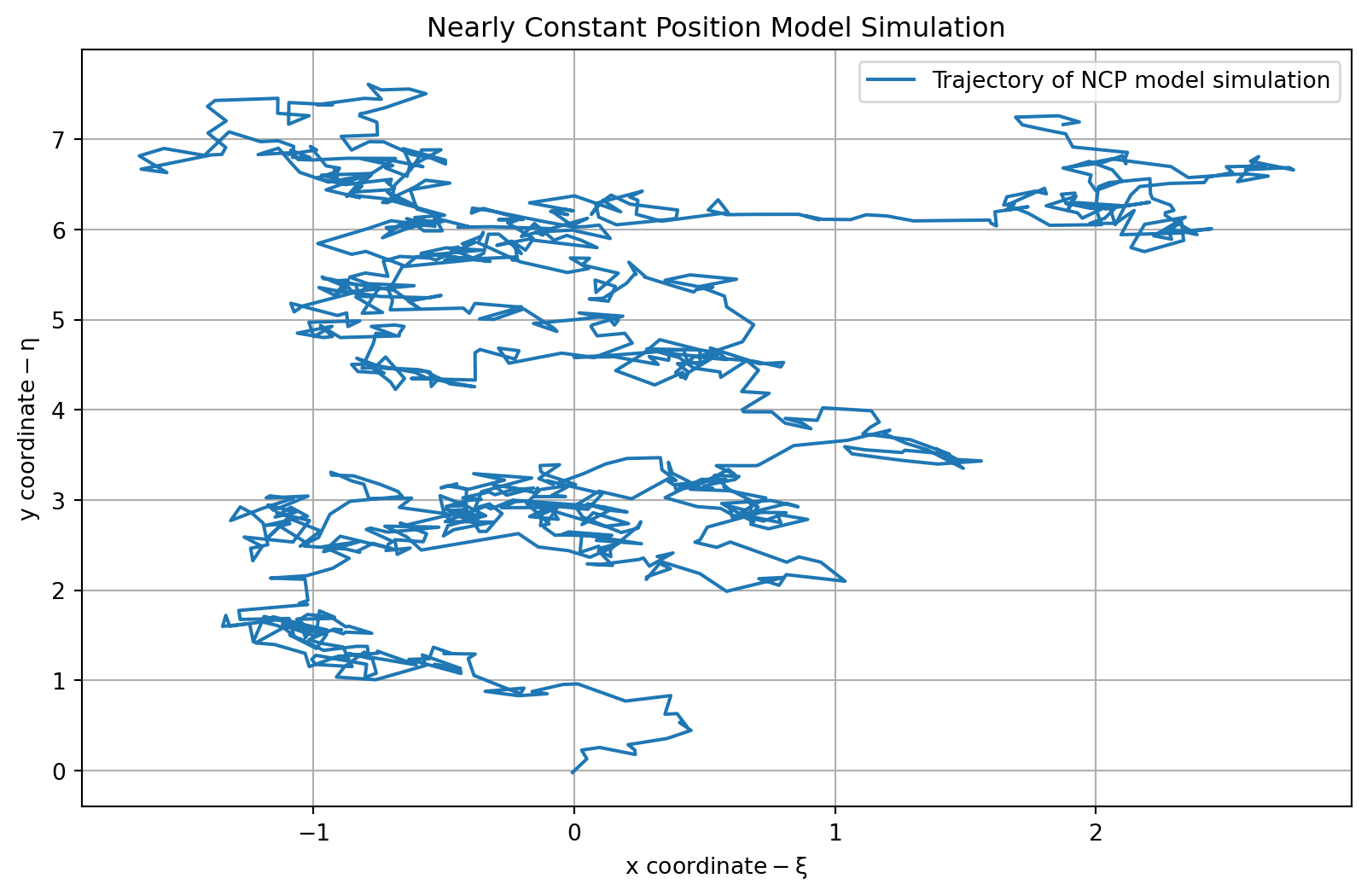
### The nearly constant position (NCP) model
In the NCP model, we assume that the target is stationary.
$$
x(t) = \begin{bmatrix} \xi(t) \\ \eta(t) \end{bmatrix}
$$ {#eq-ncp-model-state-vector}
- our models state equations is
$$
\dot{x}(t) = 0 x(t) + w(t)
$$ {#eq-ncp-model-state-equation}
- with $A= 0_{2\times 2}$ and $B=0_{2\times2}$
- our model's observation equation might be:
$$
z(t) = x(t) + v(t)
$$ {#eq-ncp-model-observation-equation}
- with $C= I_{2\times 2}$ and $D=0_{2\times2}$
```{python}
#| label: ncp-model
#| lst-label: lst-ncp-model
#| lst-cap: "NCP model simulation code"
import numpy as np
import matplotlib.pyplot as plt
maxT = 1000; # <1>
dT = 0.1; # <2>
# Define the NCP model
Ancp = np.eye(2)
Bwncp = np.eye(2)
Cncp = np.eye(2)
Dncp = np.zeros((2,2))
np.random.seed(42) # <3>
wncp = 0.1*np.random.randn(2,maxT)
vncp = 0.01*np.random.randn(2,maxT)
xncp = np.zeros(shape=(2,maxT)) # <4>
xncp[:,0] = [0,0] # <5>
for k in range(1,maxT): # <6>
xncp[:,k] = Ancp @ xncp[:,k-1] + Bwncp @ wncp[:,k-1]
zncp = Cncp @ xncp + vncp
```
1. maximum simulation time, used for all models
2. sample period used by all models (in seconds)
3. set seed for reproducibility,
4. storage
5. initial position
6. simulate the model
```{python}
#| label: fig-plot-ncp
#| fig-cap: "Plot of the NCP model simulation trajectory"
plt.figure(figsize=(10, 6))

plt.plot(zncp[0, :], zncp[1, :], label='Trajectory of NCP model simulation')
plt.title('Nearly Constant Position Model Simulation')
plt.xlabel(r'$\text{x coordinate} - \xi$')
plt.ylabel(r'$\text{y coordinate} - \eta$')
plt.legend()
plt.grid()
plt.show()
```
```{python}
#| label: lst-ncp-model-final-coordinate
print(f"Final coordinate of the trajectory: {zncp[:, -1]}") # <1>
```
1. Display the final coordinate of the trajectory
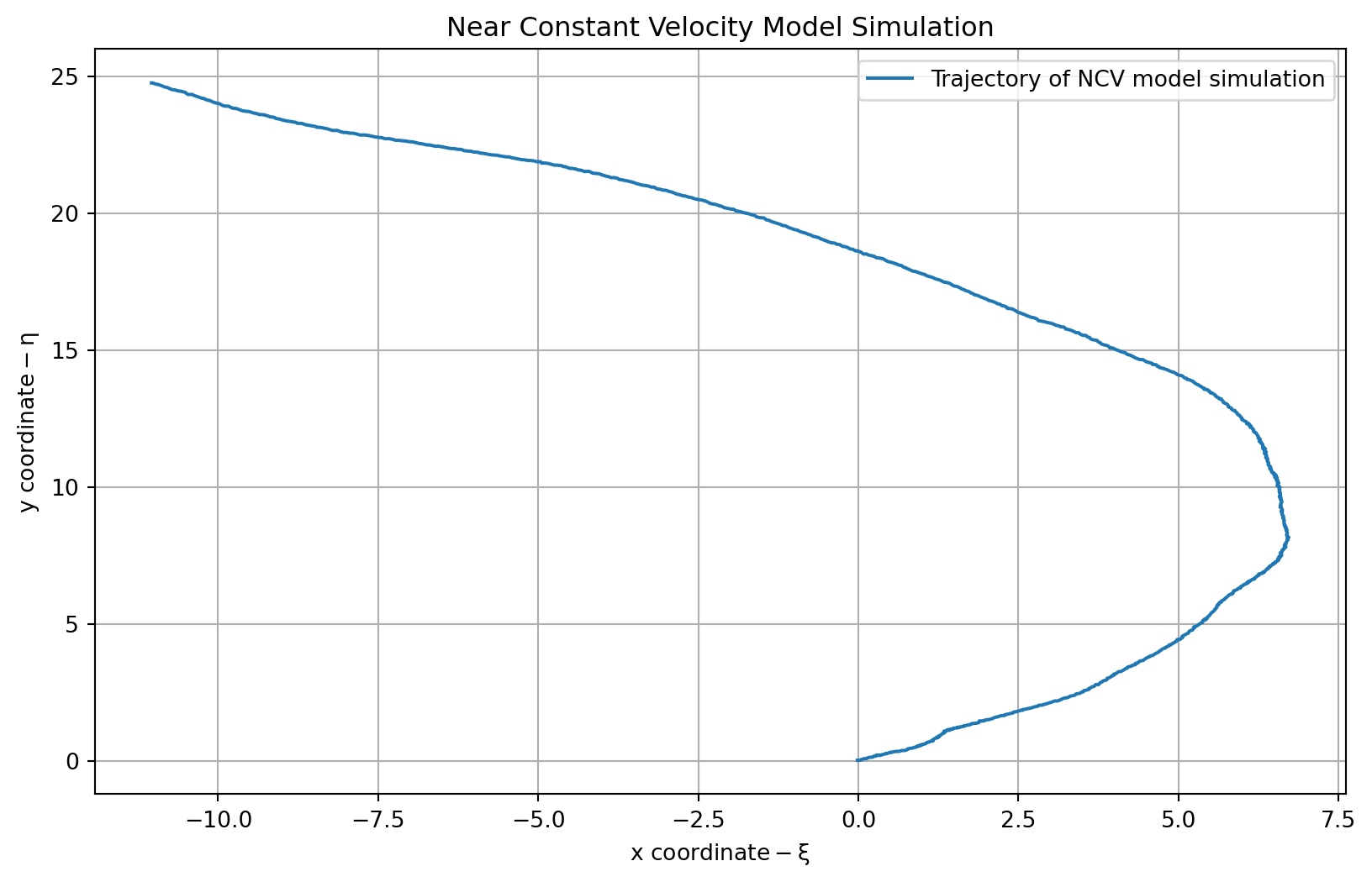
### The nearly constant velocity (NCV) model
- We now extend our target tracking model from static object to one having momentum: its velocity is nearly constant, but gets perturbed by external forces.
- The state vector is now:
$$
x(t) = \begin{bmatrix}
\xi(t) \\
\dot{\xi}(t) \\
\eta(t) \\
\dot{\eta}(t)
\end{bmatrix}
$$ {#eq-ncv-model-state-vector}
- the state equations are:
$$
\dot{x}(t) =
\underbrace{
\begin{bmatrix}
0 & 1 & 0 & 0 \\
0 & 0 & 0 & 0 \\
0 & 0 & 0 & 1 \\
0 & 0 & 0 & 0
\end{bmatrix} x(t) }_{A} +
\underbrace{
\begin{bmatrix}
0 & 0\\ 1&0 \\ 0&0 \\ 0&1
\end{bmatrix} x(t) +
\underbrace{\tilde{\omega}(t)}_{\in \mathbb{R}_{2\times 1}}
}_{\omega(t)}
$$ {#eq-ncv-model-state-equation}
- the observation equation might be:
$$
z(t) =
\underbrace{
\begin{bmatrix}
1 & 0 & 0 & 0 \\
0 & 0 & 1 & 0
\end{bmatrix}}_{C} x(t) + \nu(t)
$$ {#eq-ncv-model-observation-equation}
```{python}
#| label: ncv-model
#| lst-label: lst-ncv-model
#| lst-cap: "NCV model simulation code"
# Define the NCV model
Ancv = np.array([[1, dT, 0, 0],
                  [0, 1, 0, 0],
                  [0, 0, 1, dT],
                  [0, 0, 0, 1]])
Bwncv = np.array([[dT**2/2, 0],
                  [dT, 0],
                  [0, dT**2/2],
                  [0, dT]])
Cncv = np.array([[1, 0, 0, 0],
                 [0, 0, 1, 0]])
Dncv = np.zeros((2, 2))

np.random.seed(0)                      # Don't change this line
wncv = 0.1*np.random.randn(2,maxT)
vncv = 0.01*np.random.randn(2,maxT)

xncv = np.zeros((4,maxT))               # storage
xncv[:,0] = [0,0.1,0,0.1]               # initial position, velocity

#xncp = np.zeros(shape=(2,maxT))         # storage
#xncp[:,0] = [0,0]                       # initial posn.

for k in range(1,maxT):                 # simulate model
  xncv[:,k] = Ancv @ xncv[:,k-1] + Bwncv @ wncv[:,k-1]

zncv = Cncv @ xncv + vncv
```
```{python}
#| label: fig-plot-ncv
#| fig-cap: "Plot of the NCV model simulation trajectory"
# Plot the results
plt.figure(figsize=(10, 6))
plt.plot(zncv[0, :], zncv[1, :], label='Trajectory of NCV model simulation')
plt.title('Near Constant Velocity Model Simulation')
plt.xlabel(r'$\text{x coordinate} - \xi$')
plt.ylabel(r'$\text{y coordinate} - \eta$')
plt.legend()
plt.grid()
plt.show()
```
```{python}
#| label: lst-ncv-model-final-coordinate
print(f"Final coordinate of the trajectory: {zncv[:, -1]}") # <1>
```
1. Display the final coordinate of the trajectory
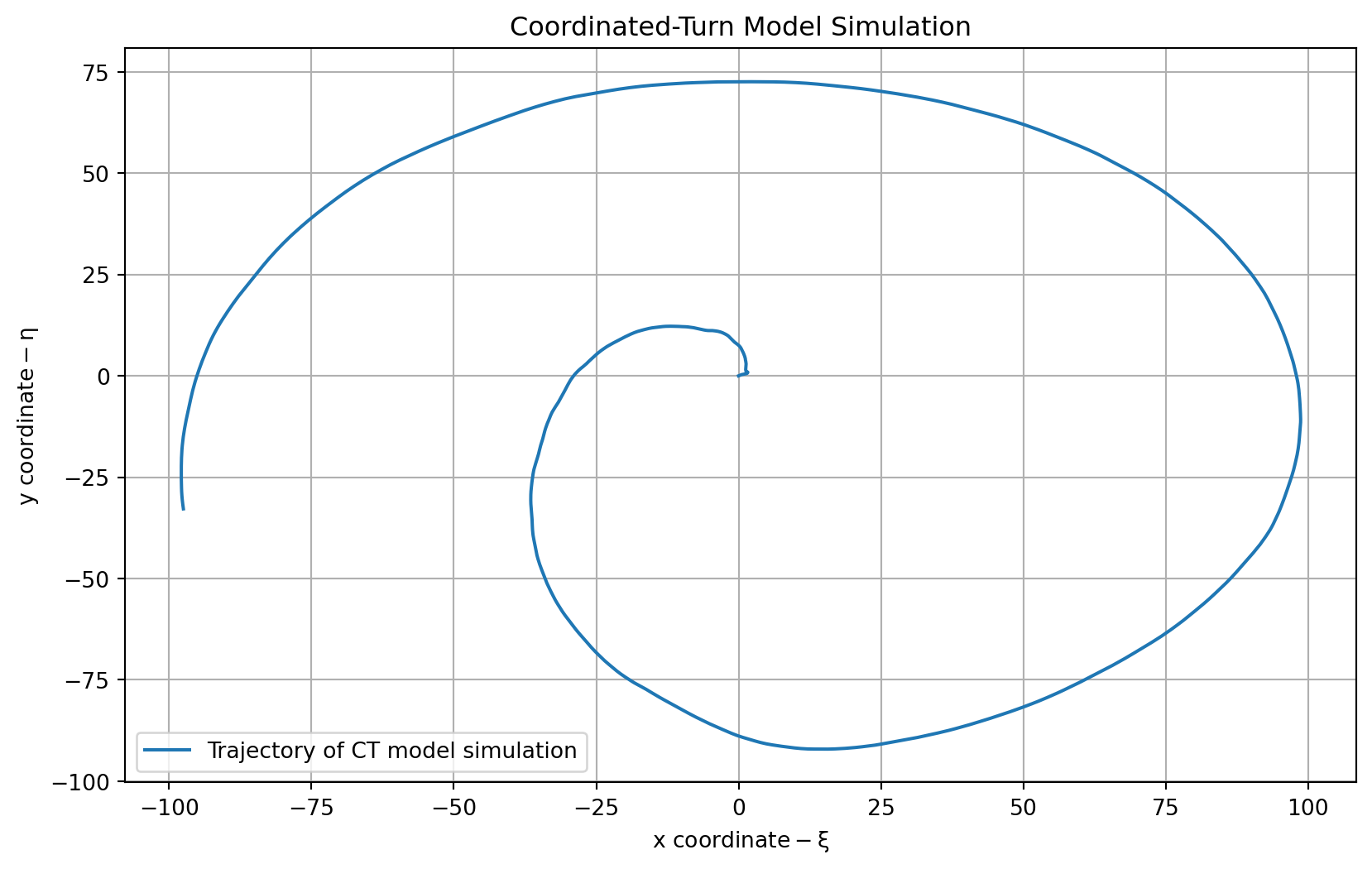
### The coordinated-turn model
We now extend our target tracking model from one having momentum to one moving a **constant angular velocity** $\Omega$
$$
\ddot{\xi}(t) = -\Omega\dot{\eta}(t) \qquad \ddot{\eta}(t) = \Omega\dot{\xi}(t)
$$ {#eq-ct-model-acceleration-equations}
- The state vector is now:
$$
x(t) = \begin{bmatrix}
\xi(t) \\
\dot{\xi}(t) \\
\eta(t) \\
\dot{\eta}(t)
\end{bmatrix}
$$ {#eq-ct-model-state-vector}
- the state equations are:
$$
\dot{x}(t) =
\underbrace{
\begin{bmatrix}
0 & 1 & 0 & 0 \\
0 & 0 & 0 & -\Omega \\
0 & 0 & 0 & 1 \\
0 & \Omega & 0 & 1
\end{bmatrix} x(t) }_{A} +
\underbrace{
\begin{bmatrix}
0 & 0\\ 1&0 \\ 0&0 \\ 0&1
\end{bmatrix} x(t) +
\underbrace{\tilde{\omega}(t)}_{\in \mathbb{R}_{2\times 1}}
}_{\omega(t)}
$$ {#eq-ct-model-state-equation}
- the observation equation might be:
$$
z(t) =
\underbrace{
\begin{bmatrix}
1 & 0 & 0 & 0 \\
0 & 0 & 1 & 0
\end{bmatrix}}_{C} x(t) + \nu(t)
$$ {#eq-ct-model-observation-equation}
```{python}
# Define the coordinated-turn model
import numpy as np
from scipy.signal import StateSpace, lsim

# Parameters
W = 0.01
A = np.array([
    [0, 1, 0, 0],
    [0, 0, 0, -W],
    [0, 0, 0, 1],
    [0, W, 0, 0]
])
Bw = np.array([
    [0, 0],
    [1, 0],
    [0, 0],
    [0, 1]
])
C = np.array([
    [1, 0, 0, 0],
    [0, 0, 1, 0]
])
D = np.zeros((2, 2))

# Create CT state-space model
ct = StateSpace(A, Bw, C, D)

# Time vector and noise
np.random.seed(0)  # Match Octave's `randn("state", 0)`
tct = np.arange(1000) * 1.0
wct = 0.01  * np.random.randn(1000, 2)  # shape (n_samples, n_inputs)
vct = 0.001 * np.random.randn(1000, 2)

# Simulate system
_, yout, _ = lsim(ct, U=wct, T=tct)

# Add sensor noise
zct = yout + vct
```
```{python}
# Plot the results
plt.figure(figsize=(10, 6))
plt.plot(zct[:, 0], zct[:, 1], label='Trajectory of CT model simulation')
plt.title('Coordinated-Turn Model Simulation')
plt.xlabel(r'$\text{x coordinate} - \xi$')
plt.ylabel(r'$\text{y coordinate} - \eta$')
plt.legend()
plt.grid()
plt.show()
```
```{python}
# Display the final coordinate of the trajectory
print(f"Final coordinate of the trajectory: {zct[-1, :]}")
```
::: {.callout-tip collapse="true"}
### Overthinking the CT model
since
question why not $\ddot{\eta}(t) = \dot{\xi}(t) = 0$?
so am I correct that we should have the following state vector?
$$
x(t) = \begin{bmatrix}
\xi(t) \\
\dot{\xi}(t) \\
\eta(t) \\
\dot{\eta}(t) \\
\ddot{\xi}(t) \\
\ddot{\eta}(t)
\end{bmatrix}
$$ {#eq-ct-model-state-vector-extended}
and the state equations are:
$$
\dot{x}(t) =
\underbrace{
\begin{bmatrix}
0 & 1 & 0 & 0 & 0 & 0 \\
0 & 0 & 0 & 0 & 1 & -\Omega \\
0 & 0 & 0 & 0 & 0 & 0 \\
0 & 0 & 0 & 0 & 0 & 0 \\
0 & 0 & \Omega & 0 & 0 & 0 \\
0 & 0 & 0 & 0 & 0 & 0
\end{bmatrix} x(t) }_{A} +
\underbrace{
\begin{bmatrix}
0 & 0 & 0 & 0\\
1 & 0 & 0 & 0 \\
0 & 0 & 0 & 0 \\
0 & 1 & 0 & 0 \\
0 & 0 & 0 & 0 \\
0 & 0 & 0 & 0
\end{bmatrix} \tilde{\omega}(t)}_{\tilde{\omega}(t)}
$$ {#eq-ct-model-state-equation-extended}
So while this took a while to formulate, it turns out that the CT model is fine. There were a number of factors contributing to my confusion.
1. The fact that this is a constant angular velocity model, so the acceleration is not zero.
- what changes is the direction and not size of the velocity vector.
- I initially didn't notice that the angular velocity is constant by definition.
2. I recalled that we need to split the velocity into two orthogonal components over time
3. The frame of reference is not explained explicitly.
- If we are in the object's frame of reference, then the angular velocity components are constant.
- If we are in the world's frame of reference, then everything is more complicated and the angular velocity components are changing sinusoidally.
4. There are a bunch of apparent forces/motions involved in circular motion on a spherical surface that surfaced in my mind.... Before I was able to make things more precise and clear.
5. How first order state representation vectors work, this is what convinced me the formulation is indeed correct and that my idea is most likely to be wrong!
- the idea is simple in @eq-ct-model-state-equation we have the first derivative of the state vector $x(t)$, which is a vector of position and velocity. The acceleration @eq-ct-model-acceleration-equations have been incorporated into the state vector.
- We can recover them by taking the second derivative of the state vector!
:::