137 Lesson 1.3.6: Continuous-time dynamic systems having random inputs

137.1 Setting up the assumptions

• For continuous-time systems we have:

  \dot{x}(t) = A x(t) + B_u u(t) + B_w w(t)

  where A, B_u and B_w are assumed to be known and constant¹ and:

  • x(t): State vector, a random process.
  • u(t): Deterministic control inputs.
  • w(t): Noise driving the process (process noise), a random process.

• Further: \begin{aligned} \mathbb{E}[x(0)] &= \bar{x}(0)& \mathbb{E}\left[(x(0)-\bar{x}(0))(x(0)-\bar{x}(0))^T\right] &= \Sigma_{\tilde{x}}(0)\\ \mathbb{E}[w(t)] &= 0 &\mathbb{E}\left[w(t)w(\tau)^T\right] &= S_w\,\delta(t-\tau). \end{aligned}

• S_w is the spectral density of w(t).

spectral density

137.2 Propagation of the mean

• Easiest analysis is to discretize model; then, use results obtained earlier for discrete-time systems letting \Delta t \to 0.
• We drop deterministic inputs u(t) from the model for simplicity. ²
• Starting with the discrete case, we have:

\begin{aligned} \bar{x}_k &= A_d \bar{x}_{k-1} + B_d u_{k-1} \\ A_d &= e^{A\Delta t} \approx I + A\Delta t + \mathcal{O}(\Delta t^2). \end{aligned}

• Let \Delta t \to 0 and consider case when u_k = 0 for all k.

\begin{aligned} \bar{x}_k &= (A\Delta t + I)\bar{x}_{k-1} \\ \frac{\bar{x}_k - \bar{x}_{k-1}}{\Delta t} &= A\bar{x}_{k-1}. \end{aligned}

• As \Delta t \to 0 \qquad \dot{\bar{x}}(t) = A\bar{x}(t) as we might expect.

137.3 Summarizing propagation of the mean

• We add back in the influence of u(t), skipping the full derivation here for simplicity.

Note

Overall, the mean propagation for continuous-time dynamic systems having random inputs is:

\begin{aligned} \bar{x}(0)& \;\text{: Given} \\ \dot{\bar{x}}(t) &= A\bar{x}(t) + B_u u(t). \end{aligned}

Simulation of a deterministic system and simulation of the mean value of the state for a stochastic system are treated the same way.

137.4 Variations about the mean

• The result for discrete-time systems was:

\Sigma_{\tilde{x},k} = A_d \Sigma_{\tilde{x},k-1} A_d^T + \Sigma_{\tilde{w}}.

• But, we need a way to relate discrete \Sigma_{\tilde{w}} to a continuous spectral density S_w before we can proceed.
• Recall the discrete system response in terms of continuous system matrices:

\begin{aligned} x_k &= e^{A\Delta t}x_{k-1} + \int_{(k-1)\Delta t}^{k\Delta t} e^{A(k\Delta t-\tau)} B_w w(\tau)\,d\tau \\ &= e^{A\Delta t}x_{k-1} + w_{k-1}. \end{aligned}

• The integral explicitly accounts for variations in the noise during \Delta t. We have:

w_{k-1} = \int_{(k-1)\Delta t}^{k\Delta t} e^{A(k\Delta t-\tau)} B_w w(\tau)\,d\tau.

137.5 Evaluating \Sigma_{\tilde{w}}

• Recall, w_k is discrete white noise having covariance:

  \mathbb{E}[w_k w_l^T] = \begin{cases} \Sigma_{\tilde{w}}, & k=l \\ 0, & k\neq l \end{cases}

• Form outer product using w_{k-1} from prior slide to get equivalent \Sigma_{\tilde{w}}:

\begin{aligned} \Sigma_{\tilde{w}} &= \mathbb{E}\left[\left(\int_{(k-1)\Delta t}^{k\Delta t} e^{A(k\Delta t-\tau)}B_w w(\tau)\,d\tau\right) \left(\int_{(k-1)\Delta t}^{k\Delta t} e^{A(k\Delta t-\gamma)}B_w w(\gamma)\,d\gamma\right)^T\right] \\ &= \mathbb{E}\left[\int_{(k-1)\Delta t}^{k\Delta t}\int_{(k-1)\Delta t}^{k\Delta t} e^{A(k\Delta t-\tau)}B_w w(\tau)w(\gamma)^T B_w^T e^{A^T(k\Delta t-\gamma)}\,d\tau\,d\gamma\right] \end{aligned}

• Big ugly mess but has two saving graces:
  1. Expectation can go inside integrals.
  2. \mathbb{E}[w(\tau)w(\gamma)^T] = S_w\,\delta(\tau-\gamma) \implies one of the integrals drops out.

137.6 The solution for \Sigma_{\tilde{w}}

• So, we have:

\Sigma_{\tilde{w}} = \int_{(k-1)\Delta t}^{k\Delta t} e^{A(k\Delta t-\tau)} B_w S_w B_w^T e^{A^T(k\Delta t-\tau)}\,d\tau.

• While S_w may have a simple form, \Sigma_{\tilde{w}} will be a full matrix in general.

• One approach to solving the integral is to approximate.

  • As \Delta t \to 0, then k\Delta t - \tau \to 0 and e^{A(k\Delta t-\tau)} \approx I + A(k\Delta t-\tau) + \cdots

  • That is, e^{A(k\Delta t-\tau)} \approx I. Then,

  \Sigma_{\tilde{w}} \approx (B_w S_w B_w^T)\,\Delta t.

• We will see a better method to evaluate \Sigma_{\tilde{w}} when \Delta t \neq 0, but for now we continue with this result to determine the continuous-time system covariance propagation.

137.7 The solution for \Sigma_{\tilde{x},k}

• We now substitute \Sigma_{\tilde{w}} \approx B_w S_w B_w^T\Delta t and A_d \approx (I + A\Delta t) into the covariance-propagation equation:

  \begin{aligned} \Sigma_{\tilde{x},k} &= A_d \Sigma_{\tilde{x},k-1} A_d^T + \Sigma_{\tilde{w}} \\ & \approx (I + A\Delta t)\Sigma_{\tilde{x},k-1}(I + A\Delta t)^T + B_w S_w B_w^T\Delta t \\ &= \Sigma_{\tilde{x},k-1} + \Delta t\left(A\Sigma_{\tilde{x},k-1} + \Sigma_{\tilde{x},k-1}A^T + B_w S_w B_w^T\right) + \mathcal{O}(\Delta t^2) \\ \frac{\Sigma_{\tilde{x},k} - \Sigma_{\tilde{x},k-1}}{\Delta t} &= A\Sigma_{\tilde{x},k-1} + \Sigma_{\tilde{x},k-1}A^T + B_w S_w B_w^T + \mathcal{O}(\Delta t). \end{aligned}

• As \Delta t \to 0, \dot{\Sigma}_{\tilde{x}}(t) = A\Sigma_{\tilde{x}}(t) + \Sigma_{\tilde{x}}(t)A^T + B_w S_w B_w^T, initialized with \Sigma_{\tilde{x}}(0).

137.8 Interpreting the solution for \Sigma_{\tilde{x},k}

• Covariance: \dot{\Sigma}_{\tilde{x}}(t) = A\Sigma_{\tilde{x}}(t) + \Sigma_{\tilde{x}}(t)A^T + B_w S_w B_w^T

• This is a matrix differential equation.

• Symmetric, so we don’t need to solve for every element³. Two effects:

  • A \Sigma_{\tilde{x}}(t) + \Sigma_{\tilde{x}}(t)A^T
    • Homogeneous part.
    • Contractive for stable A.
    • Reduces covariance.
  • B_w S_w B_w^T
    • Impact of process noise.
    • Tends to increase covariance.

• Steady-state solution: Effects balance for systems having constant matrices A, B_w, S_w and stable A. A\Sigma_{\tilde{x},ss} + \Sigma_{\tilde{x},ss}A^T + B_w S_w B_w^T = 0.

• This is a continuous-time Lyapunov equation. In Octave, lyap.m.

137.9 Summarizing propagation of the covariance

• So, after a short derivation, we now have the solution for how the uncertainty of the state is propagated over time.

Note

The covariance propagation is:

\begin{aligned} \Sigma_{\tilde{x}}(0)&\;\text{: Given} \\ \dot{\Sigma}_{\tilde{x}}(t) &= \underbrace{A\Sigma_{\tilde{x}}(t) + \Sigma_{\tilde{x}}(t)A^T}_{\text{homogeneous term}} + \underbrace{B_w S_w B_w^T}_{\text{driving term}}. \end{aligned}

137.10 An example, solving for steady-state

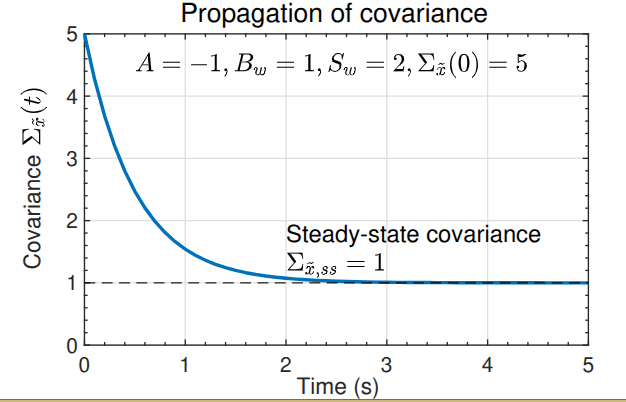
• \dot{x}(t) = Ax(t) + B_w w(t), where A and B_w are scalars.
• Then, \dot{\Sigma}_{\tilde{x}} = 2A\Sigma_{\tilde{x}} + B_w^2 S_w the solution to this ODE is: \Sigma_{\tilde{x}}(t) = \frac{B_w^2 S_w}{2A}\left(e^{2At} - 1\right) + \Sigma_{\tilde{x}}(0)e^{2At}.
• If A < 0 (stable) then the initial condition contribution goes to zero and: \Sigma_{\tilde{x},ss} = -\frac{B_w^2 S_w}{2A}.
• Increased \Sigma_{\tilde{x},ss} as more noise added via the B_w^2 S_w term; decreased \Sigma_{\tilde{x},ss} as A becomes “more stable”.
• Example shown to the right.

137.11 Summary

• With deterministic state-space systems, we can simulate a model and have no uncertainty regarding the state trajectory.
• With stochastic state-space systems, we instead track the mean and covariance of the RV representing the state at every point in time.
• We learned how to update the mean and covariance: \begin{aligned} \dot{\bar{x}}(t) &= A\bar{x}(t) + B_u u(t) \\ \dot{\Sigma}_{\tilde{x}}(t) &= A\Sigma_{\tilde{x}}(t) + \Sigma_{\tilde{x}}(t)A^T + B_w S_w B_w^T. \end{aligned}
• The true state x(t) is expected to be within \bar{x}(t) \pm 3\sqrt{\operatorname{diag}(\Sigma_{\tilde{x}}(t))} approximately 99.7\% of the time if the model is correct and noises are Gaussian.

---

1. can generalize later if needed

2. They affect only the mean, and in known ways, and we add their influence back in later.

3. just one triangle of the matrix