data("PlantGrowth")
#?PlantGrowth
head(PlantGrowth)
weight group
1 4.17 ctrl
2 5.58 ctrl
3 5.18 ctrl
4 6.11 ctrl
5 4.50 ctrl
6 4.61 ctrlANOVA, Bayesian statistics, R programming, statistical modeling, Analysis of Variance
As an example of a one-way ANOVA, we’ll look at the Plant Growth data in R.
data("PlantGrowth")
#?PlantGrowth
head(PlantGrowth) weight group
1 4.17 ctrl
2 5.58 ctrl
3 5.18 ctrl
4 6.11 ctrl
5 4.50 ctrl
6 4.61 ctrlWe first load the dataset (Listing 43.1)
Because the explanatory variable group is a factor and not continuous, we choose to visualize the data with box plots rather than scatter plots.
boxplot(weight ~ group, data=PlantGrowth)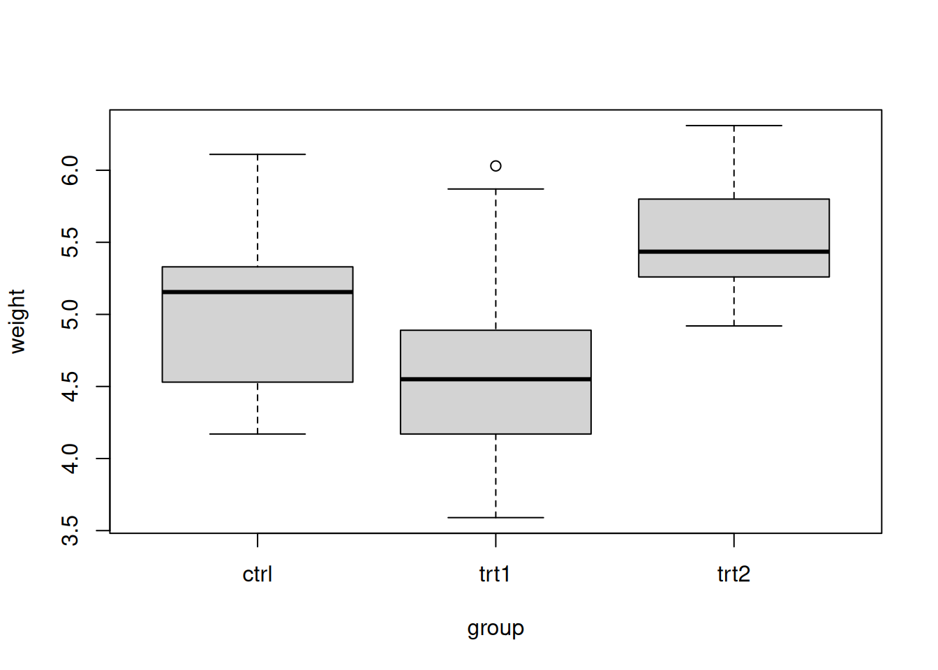
The box plots summarize the distribution of the data for each of the three groups. It appears that treatment 2 has the highest mean yield. It might be questionable whether each group has the same variance, but we’ll assume that is the case.
Again, we can start with the reference analysis (with a noninformative prior) with a linear model in R.
lmod = lm(weight ~ group, data=PlantGrowth)
summary(lmod)
Call:
lm(formula = weight ~ group, data = PlantGrowth)

Residuals:
    Min      1Q  Median      3Q     Max
-1.0710 -0.4180 -0.0060  0.2627  1.3690

Coefficients:
            Estimate Std. Error t value Pr(>|t|)
(Intercept)   5.0320     0.1971  25.527   <2e-16 ***
grouptrt1    -0.3710     0.2788  -1.331   0.1944
grouptrt2     0.4940     0.2788   1.772   0.0877 .
---
Signif. codes:  0 '***' 0.001 '**' 0.01 '*' 0.05 '.' 0.1 ' ' 1

Residual standard error: 0.6234 on 27 degrees of freedom
Multiple R-squared:  0.2641,    Adjusted R-squared:  0.2096
F-statistic: 4.846 on 2 and 27 DF, p-value: 0.01591anova(lmod)Analysis of Variance Table
Response: weight
Df Sum Sq Mean Sq F value Pr(>F)
group 2 3.7663 1.8832 4.8461 0.01591 *
Residuals 27 10.4921 0.3886
---
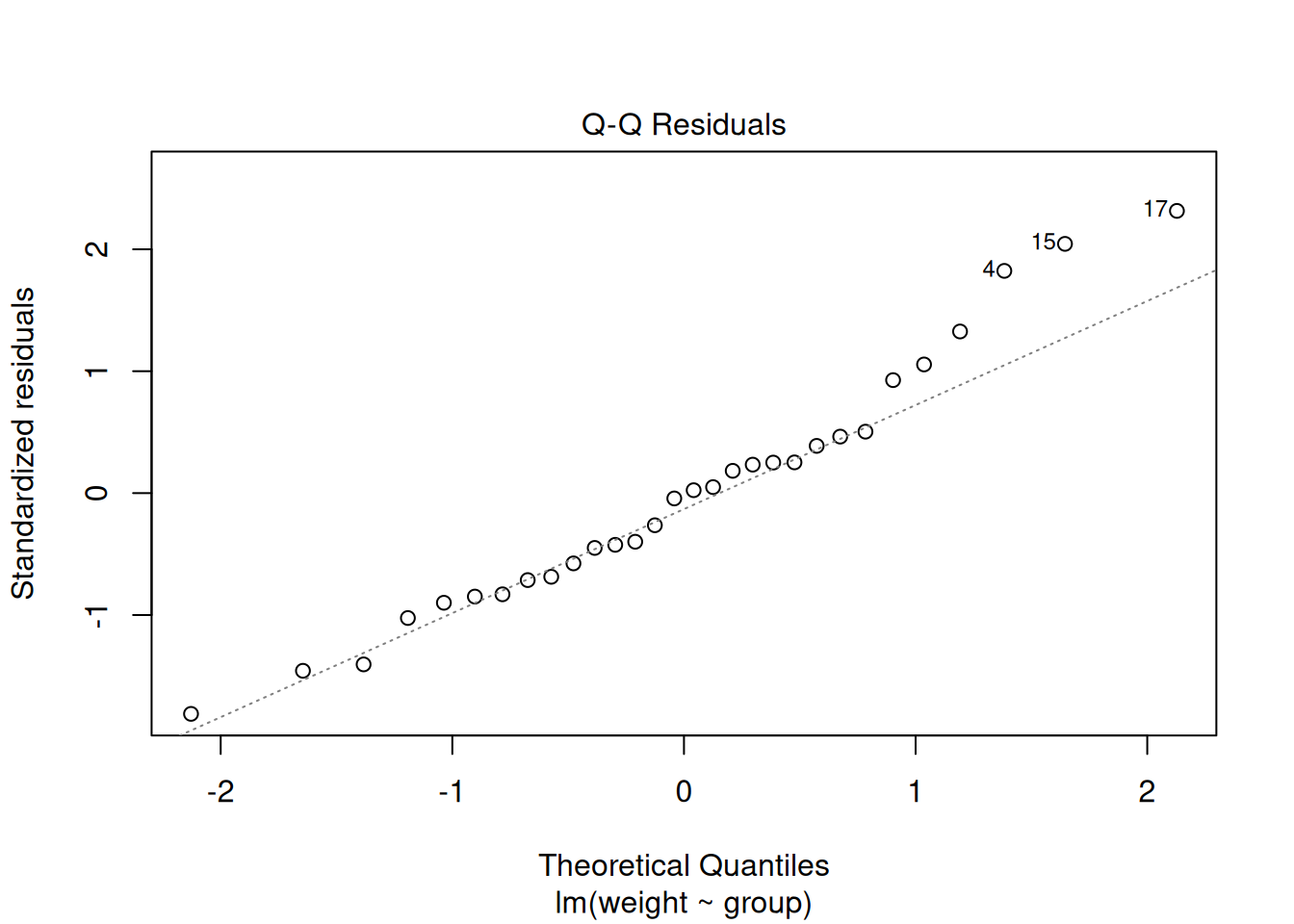
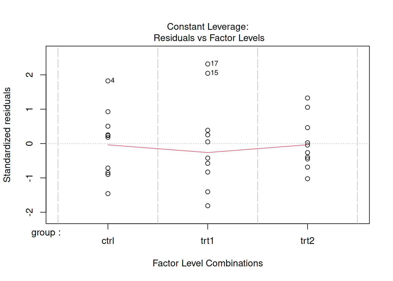
Signif. codes: 0 '***' 0.001 '**' 0.01 '*' 0.05 '.' 0.1 ' ' 1plot(lmod) # for graphical residual analysis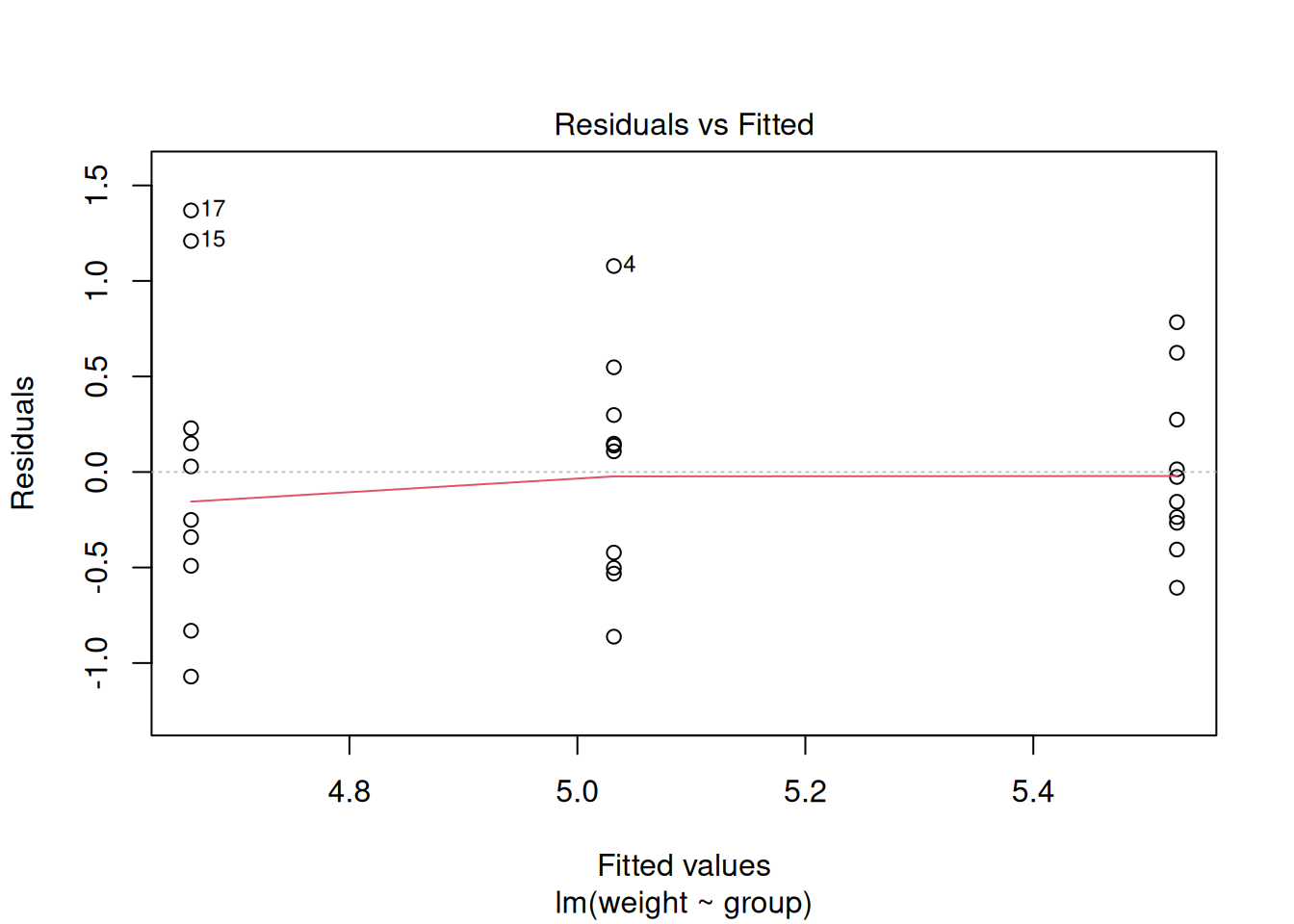
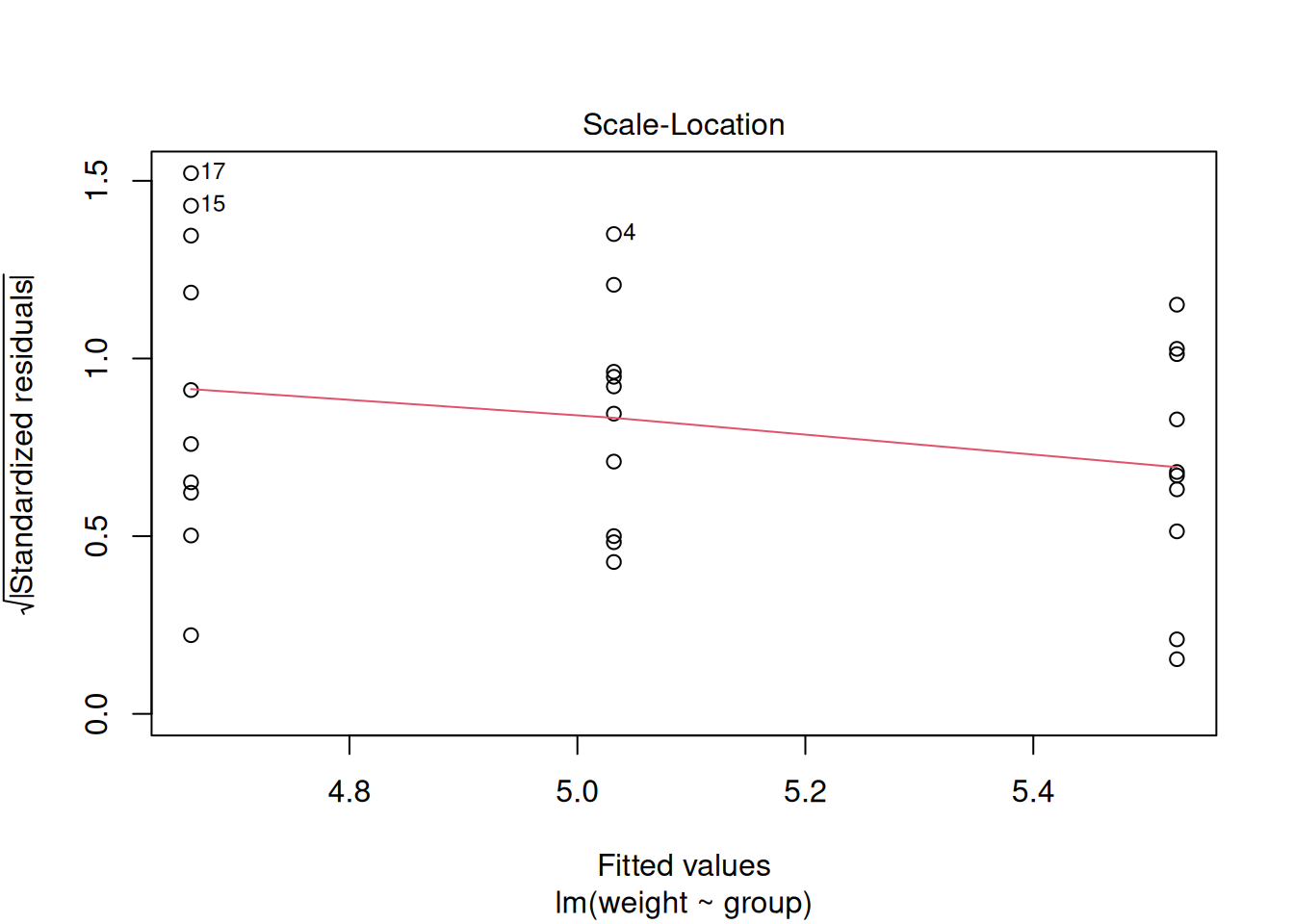
The default model structure in R is the linear model with dummy indicator variables. Hence, the “intercept” in this model is the mean yield for the control group. The two other parameters are the estimated effects of treatments 1 and 2. To recover the mean yield in treatment group 1, you would add the intercept term and the treatment 1 effect. To see how R sets the model up, use the model.matrix(lmod) function to extract the X matrix.
The anova() function in R compares variability of observations between the treatment groups to variability within the treatment groups to test whether all means are equal or whether at least one is different. The small p-value here suggests that the means are not all equal.
Let’s fit the cell means model in JAGS.
library("rjags")mod_string = " model {
for (i in 1:length(y)) {
y[i] ~ dnorm(mu[grp[i]], prec)
}
for (j in 1:3) {
mu[j] ~ dnorm(0.0, 1.0/1.0e6)
}
prec ~ dgamma(5/2.0, 5*1.0/2.0)
sig = sqrt( 1.0 / prec )
} "
set.seed(82)
str(PlantGrowth)'data.frame': 30 obs. of 2 variables:
$ weight: num 4.17 5.58 5.18 6.11 4.5 4.61 5.17 4.53 5.33 5.14 ...
$ group : Factor w/ 3 levels "ctrl","trt1",..: 1 1 1 1 1 1 1 1 1 1 ...data_jags = list(y=PlantGrowth$weight,
grp=as.numeric(PlantGrowth$group))
params = c("mu", "sig")
inits = function() {
inits = list("mu"=rnorm(3,0.0,100.0), "prec"=rgamma(1,1.0,1.0))
}
mod = jags.model(textConnection(mod_string), data=data_jags, inits=inits, n.chains=3)Compiling model graph
Resolving undeclared variables
Allocating nodes
Graph information:
Observed stochastic nodes: 30
Unobserved stochastic nodes: 4
Total graph size: 74
Initializing modelupdate(mod, 1e3)
mod_sim = coda.samples(model=mod,
variable.names=params,
n.iter=5e3)
mod_csim = as.mcmc(do.call(rbind, mod_sim)) # combined chainsAs usual, we check for convergence of our MCMC.
par(mar = c(2.5, 1, 2.5, 1))
plot(mod_sim)

gelman.diag(mod_sim)
Potential scale reduction factors:
Point est. Upper C.I.
mu[1] 1 1
mu[2] 1 1
mu[3] 1 1
sig 1 1
Multivariate psrf
1autocorr.diag(mod_sim) mu[1] mu[2] mu[3] sig
Lag 0 1.000000000 1.00000000 1.000000000 1.0000000000
Lag 1 0.014336180 0.02199016 0.012807552 0.0885297420
Lag 5 -0.001671659 -0.01784307 -0.002987901 -0.0107120177
Lag 10 -0.014142504 -0.00703251 -0.010683217 0.0019732403
Lag 50 0.003688111 0.01469418 0.002424623 -0.0003510294effectiveSize(mod_sim) mu[1] mu[2] mu[3] sig
14780.32 15377.43 14735.34 12471.35 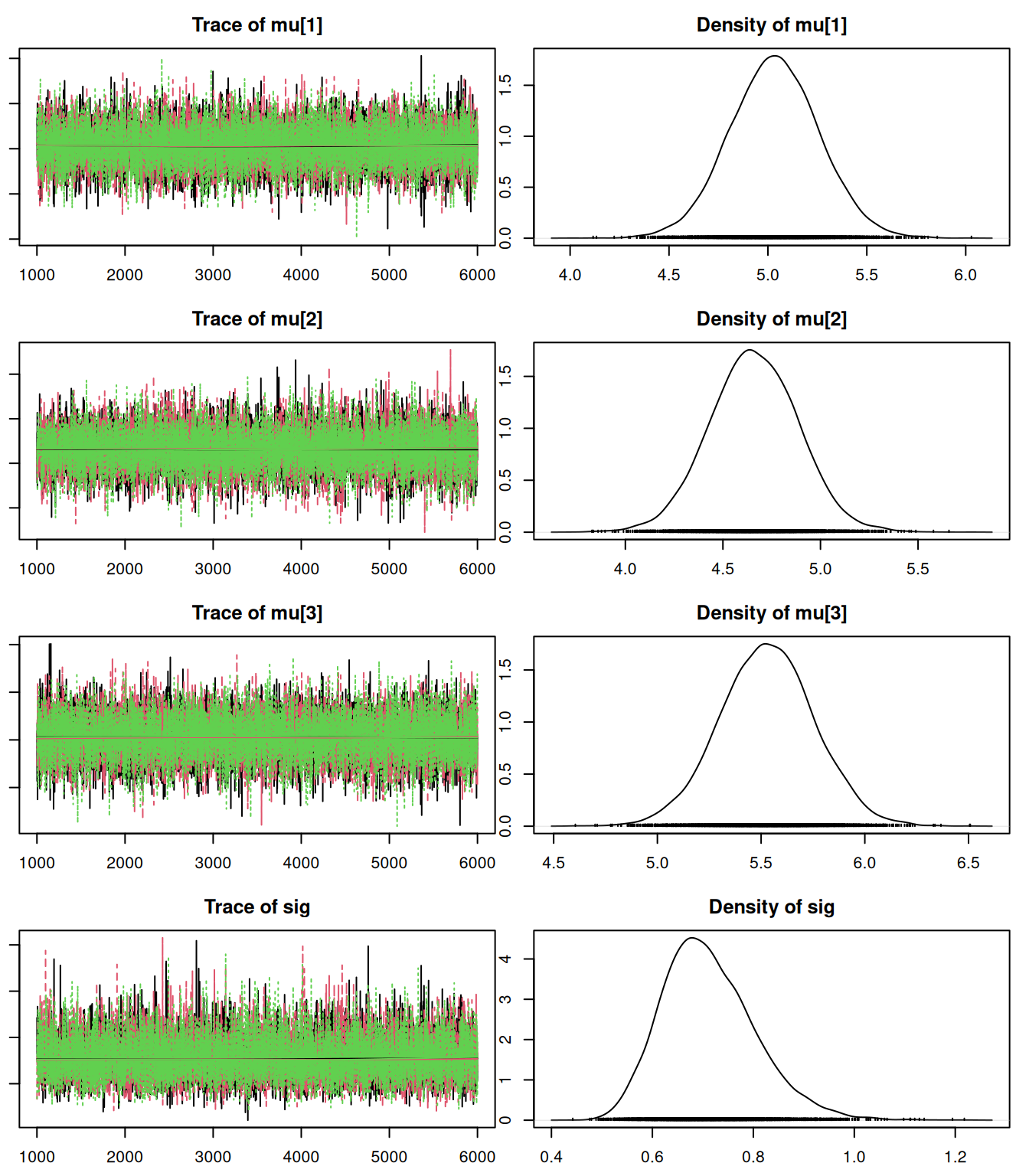
We can also look at the residuals to see if there are any obvious problems with our model choice.
(pm_params = colMeans(mod_csim)) mu[1] mu[2] mu[3] sig
5.0340778 4.6599362 5.5288313 0.7115528 yhat = pm_params[1:3][data_jags$grp]
resid = data_jags$y - yhat
plot(resid)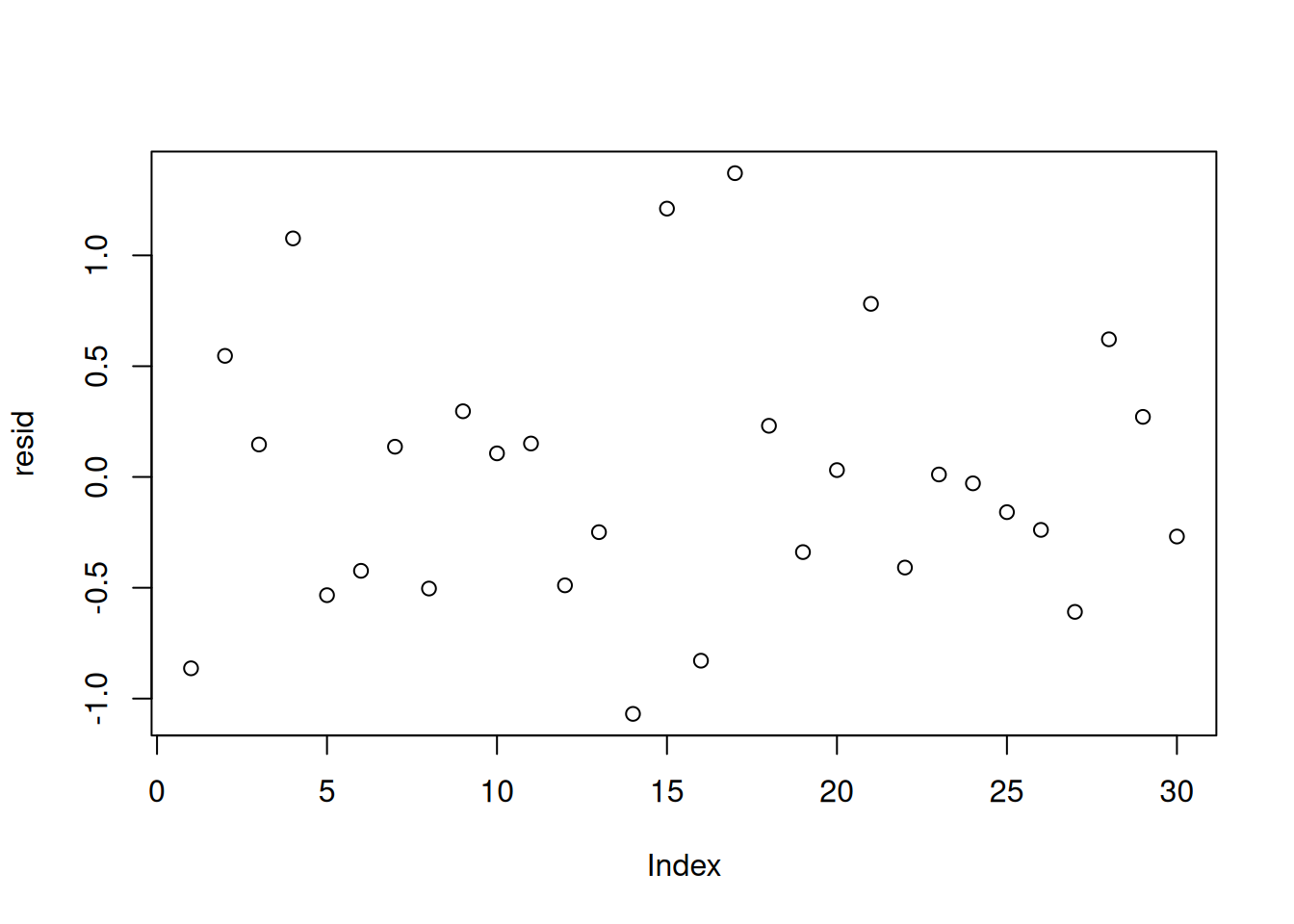
plot(yhat, resid)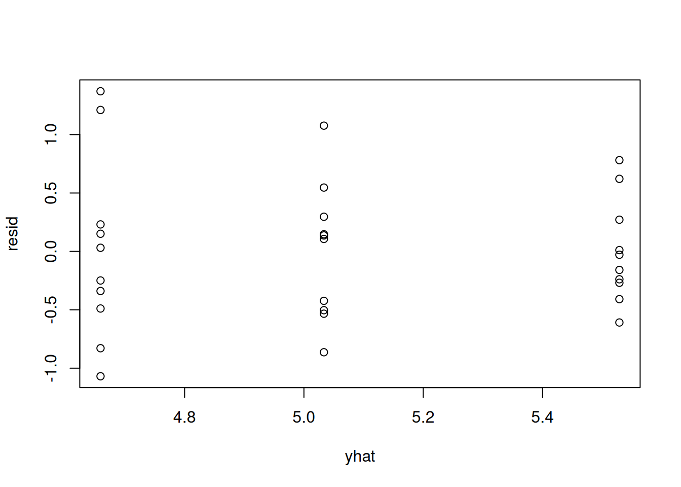
Again, it might be appropriate to have a separate variance for each group. We will have you do that as an exercise.
Let’s look at the posterior summary of the parameters.
summary(mod_sim)
Iterations = 1001:6000
Thinning interval = 1
Number of chains = 3
Sample size per chain = 5000

1. Empirical mean and standard deviation for each variable,
   plus standard error of the mean:

        Mean      SD  Naive SE Time-series SE
mu[1] 5.0341 0.22527 0.0018393      0.0018536
mu[2] 4.6599 0.22695 0.0018531      0.0018316
mu[3] 5.5288 0.22548 0.0018410      0.0018582
sig   0.7116 0.09142 0.0007464      0.0008188

2. Quantiles for each variable:

        2.5%    25%    50%   75%  97.5%
mu[1] 4.5937 4.8837 5.0327 5.184 5.4787
mu[2] 4.2165 4.5106 4.6600 4.809 5.1104
mu[3] 5.0857 5.3778 5.5305 5.679 5.9739
sig 0.5586 0.6469 0.7025 0.766 0.9164HPDinterval(mod_csim) lower upper
mu[1] 4.6085099 5.4910422
mu[2] 4.2119869 5.1055270
mu[3] 5.0753634 5.9621287
sig 0.5378479 0.8888493
attr(,"Probability")
[1] 0.95The HPDinterval() function in the coda package calculates intervals of highest posterior density for each parameter.
We are interested to know if one of the treatments increases mean yield. It is clear that treatment 1 does not. What about treatment 2?
mean(mod_csim[,3] > mod_csim[,1])[1] 0.9412There is a high posterior probability that the mean yield for treatment 2 is greater than the mean yield for the control group.
It may be the case that treatment 2 would be costly to put into production. Suppose that to be worthwhile, this treatment must increase mean yield by 10%. What is the posterior probability that the increase is at least that?
mean(mod_csim[,3] > 1.1*mod_csim[,1])[1] 0.4874667We have about 50/50 odds that adopting treatment 2 would increase mean yield by at least 10%.
Let’s explore an example with two factors. We’ll use the Warpbreaks data set in R. Check the documentation for a description of the data by typing ?warpbreaks.
data("warpbreaks")
#?warpbreaks
head(warpbreaks)
breaks wool tension
1 26 A L
2 30 A L
3 54 A L
4 25 A L
5 70 A L
6 52 A L# This chunk is for displaying the output that was previously static.
# If the static output below is preferred, this chunk can be removed
# and the static output remains unlabelled as it's not a code cell.
# For a labeled table, this chunk should generate it.
# The original file had static output here:
## breaks wool tension
## 1 26 A L
## 2 30 A L
## 3 54 A L
## 4 25 A L
## 5 70 A L
## 6 52 A L
# To make this a labeled table from code:
head(warpbreaks) breaks wool tension
1 26 A L
2 30 A L
3 54 A L
4 25 A L
5 70 A L
6 52 A Ltable(warpbreaks$wool, warpbreaks$tension)
    L M H
  A 9 9 9
  B 9 9 9
Again, we visualize the data with box plots.
boxplot(breaks ~ wool + tension, data=warpbreaks)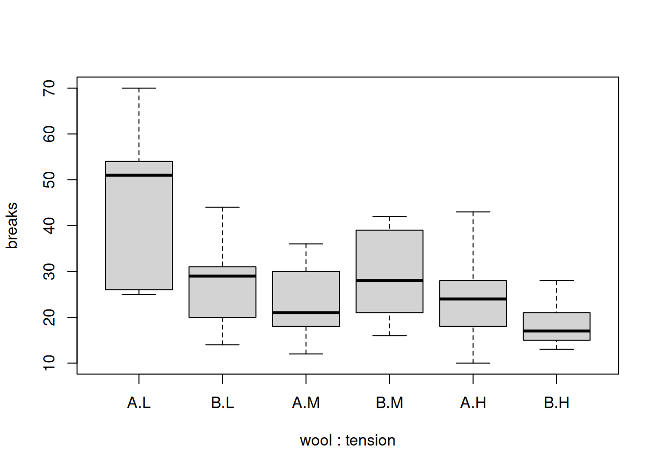
boxplot(log(breaks) ~ wool + tension, data=warpbreaks)
The different groups have more similar variance if we use the logarithm of breaks. From this visualization, it looks like both factors may play a role in the number of breaks. It appears that there is a general decrease in breaks as we move from low to medium to high tension. Let’s start with a one-way model using tension only.
mod1_string = " model {
    for( i in 1:length(y)) {
        y[i] ~ dnorm(mu[tensGrp[i]], prec)
    }

    for (j in 1:3) {
        mu[j] ~ dnorm(0.0, 1.0/1.0e6)
    }

    prec ~ dgamma(5/2.0, 5*2.0/2.0)
    sig = sqrt(1.0 / prec)
} "

set.seed(83)
str(warpbreaks)
'data.frame': 54 obs. of 3 variables:
$ breaks : num 26 30 54 25 70 52 51 26 67 18 ...
$ wool : Factor w/ 2 levels "A","B": 1 1 1 1 1 1 1 1 1 1 ...
$ tension: Factor w/ 3 levels "L","M","H": 1 1 1 1 1 1 1 1 1 2 ...data1_jags = list(y=log(warpbreaks$breaks), tensGrp=as.numeric(warpbreaks$tension))
params1 = c("mu", "sig")
mod1 = jags.model(textConnection(mod1_string), data=data1_jags, n.chains=3)Compiling model graph
Resolving undeclared variables
Allocating nodes
Graph information:
Observed stochastic nodes: 54
Unobserved stochastic nodes: 4
Total graph size: 123
Initializing modelupdate(mod1, 1e3)
mod1_sim = coda.samples(model=mod1,
variable.names=params1,
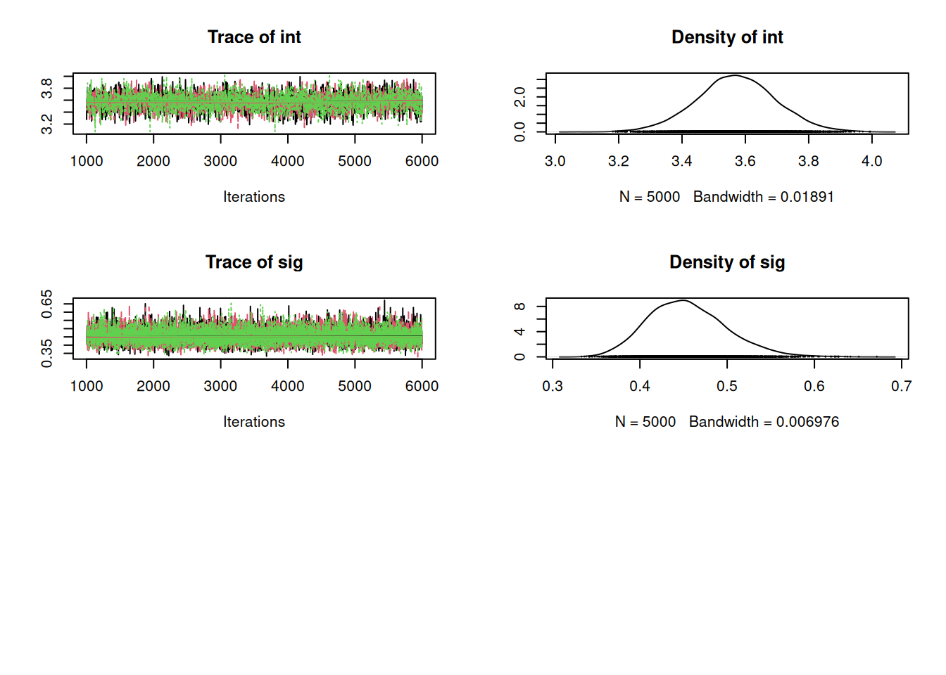
n.iter=5e3)## convergence diagnostics
plot(mod1_sim)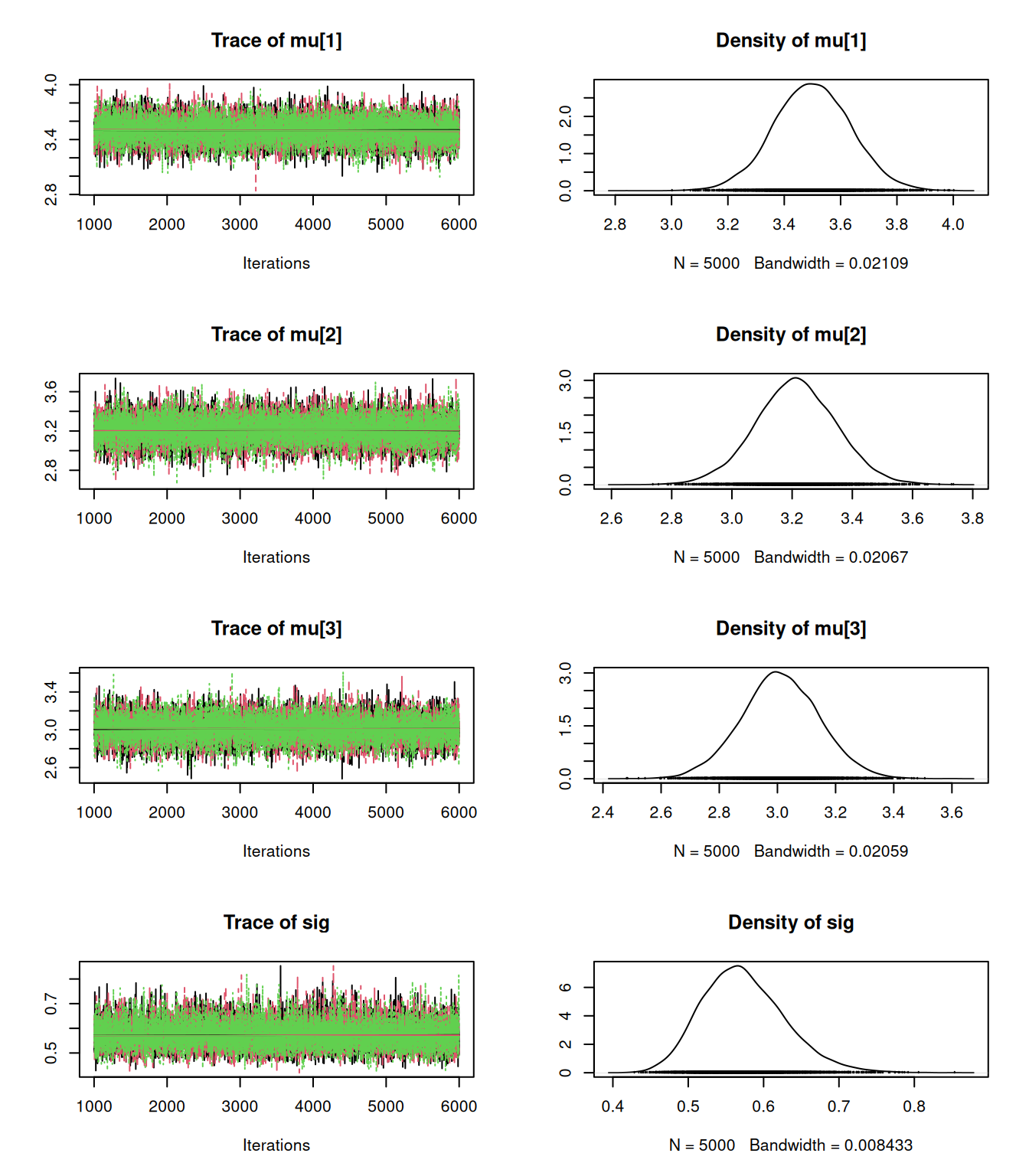
gelman.diag(mod1_sim)Potential scale reduction factors:
Point est. Upper C.I.
mu[1] 1 1
mu[2] 1 1
mu[3] 1 1
sig 1 1
Multivariate psrf
1autocorr.diag(mod1_sim) mu[1] mu[2] mu[3] sig
Lag 0 1.000000000 1.0000000000 1.000000000 1.000000000
Lag 1 0.014498409 0.0042002859 0.007874470 0.062165966
Lag 5 0.002384160 -0.0006795319 0.004896836 0.002956901
Lag 10 -0.002458494 -0.0140978451 -0.006142748 -0.004331188
Lag 50 0.003803800 0.0027780549 0.006521811 -0.007054540effectiveSize(mod1_sim) mu[1] mu[2] mu[3] sig
14662.57 15337.57 14600.33 13585.28 The 95% posterior interval for the mean of group 2 (medium tension) overlaps with both the low and high groups, but the intervals for low and high group only slightly overlap. That is a pretty strong indication that the means for low and high tension are different. Let’s collect the DIC for this model and move on to the two-way model.
dic1 = dic.samples(mod1, n.iter=1e3)With two factors, one with two levels and the other with three, we have six treatment groups, which is the same situation we discussed when introducing multiple factor ANOVA. We will first fit the additive model which treats the two factors separately with no interaction. To get the X matrix (or design matrix) for this model, we can create it in R.
X = model.matrix( ~ wool + tension, data=warpbreaks)
head(X)
(Intercept) woolB tensionM tensionH
1 1 0 0 0
2 1 0 0 0
3 1 0 0 0
4 1 0 0 0
5 1 0 0 0
6 1 0 0 0tail(X) (Intercept) woolB tensionM tensionH
49 1 1 0 1
50 1 1 0 1
51 1 1 0 1
52 1 1 0 1
53 1 1 0 1
54 1 1 0 1By default, R has chosen the mean for wool A and low tension to be the intercept. Then, there is an effect for wool B, and effects for medium tension and high tension, each associated with dummy indicator variables.
mod2_string = " model {
    for( i in 1:length(y)) {
        y[i] ~ dnorm(mu[i], prec)
        mu[i] = int + alpha*isWoolB[i] + beta[1]*isTensionM[i] + beta[2]*isTensionH[i]
    }

    int ~ dnorm(0.0, 1.0/1.0e6)
    alpha ~ dnorm(0.0, 1.0/1.0e6)
    for (j in 1:2) {
        beta[j] ~ dnorm(0.0, 1.0/1.0e6)
    }

    prec ~ dgamma(3/2.0, 3*1.0/2.0)
    sig = sqrt(1.0 / prec)
} "

data2_jags = list(y=log(warpbreaks$breaks), isWoolB=X[,"woolB"], isTensionM=X[,"tensionM"], isTensionH=X[,"tensionH"])

params2 = c("int", "alpha", "beta", "sig")

mod2 = jags.model(textConnection(mod2_string), data=data2_jags, n.chains=3)
Compiling model graph
Resolving undeclared variables
Allocating nodes
Graph information:
Observed stochastic nodes: 54
Unobserved stochastic nodes: 5
Total graph size: 243
Initializing modelupdate(mod2, 1e3)
mod2_sim = coda.samples(model=mod2,
variable.names=params2,
n.iter=5e3)## convergence diagnostics
plot(mod2_sim)
gelman.diag(mod2_sim) # Corrected from mod1_simPotential scale reduction factors:
Point est. Upper C.I.
alpha 1 1.00
beta[1] 1 1.01
beta[2] 1 1.01
int 1 1.01
sig 1 1.00
Multivariate psrf
1autocorr.diag(mod2_sim) # Corrected from mod1_sim alpha beta[1] beta[2] int sig
Lag 0 1.00000000 1.00000000 1.000000000 1.000000000 1.0000000000
Lag 1 0.49639916 0.48943458 0.494376502 0.741458618 0.0698971669
Lag 5 0.02853406 0.08397750 0.082811834 0.151667078 -0.0031975683
Lag 10 -0.00129072 0.01725858 0.016843135 0.010624860 -0.0011479978
Lag 50 0.01618153 0.01042301 0.006016021 0.008288256 0.0005444373effectiveSize(mod2_sim) # Corrected from mod1_sim alpha beta[1] beta[2] int sig
5224.047 4043.387 4299.401 2694.565 12696.771 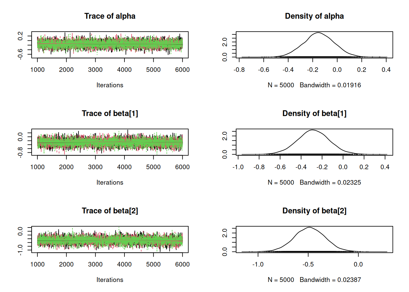
Let’s summarize the results, collect the DIC for this model, and compare it to the first one-way model.
summary(mod2_sim)
Iterations = 1001:6000
Thinning interval = 1
Number of chains = 3
Sample size per chain = 5000

1. Empirical mean and standard deviation for each variable,
   plus standard error of the mean:

           Mean      SD  Naive SE Time-series SE
alpha   -0.1550 0.12510 0.0010214       0.001734
beta[1] -0.2893 0.14991 0.0012240       0.002357
beta[2] -0.4909 0.15098 0.0012327       0.002305
int      3.5794 0.12230 0.0009986       0.002355
sig      0.4542 0.04472 0.0003651       0.000397

2. Quantiles for each variable:

           2.5%     25%     50%      75%      97.5%
alpha   -0.4018 -0.2379 -0.1547 -0.07041  0.0863790
beta[1] -0.5829 -0.3905 -0.2885 -0.18822  0.0006765
beta[2] -0.7901 -0.5905 -0.4901 -0.39053 -0.1940149
int      3.3390  3.4977  3.5789  3.66049  3.8209142
sig 0.3762 0.4229 0.4507 0.48181 0.5516939(dic2 = dic.samples(mod2, n.iter=1e3))Mean deviance: 55.61
penalty 5.213
Penalized deviance: 60.83 dic1Mean deviance: 66.64
penalty 3.997
Penalized deviance: 70.64 This suggests there is much to be gained adding the wool factor to the model. Before we settle on this model however, we should consider whether there is an interaction. Let’s look again at the box plot with all six treatment groups.
boxplot(log(breaks) ~ wool + tension, data=warpbreaks)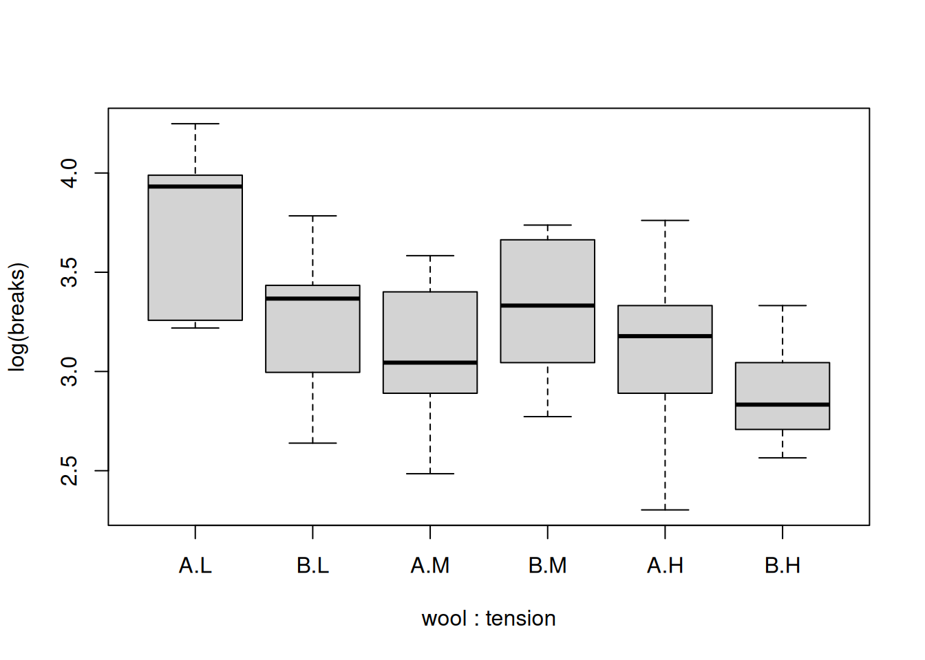
Our two-way model has a single effect for wool B and the estimate is negative. If this is true, then we would expect wool B to be associated with fewer breaks than its wool A counterpart on average. This is true for low and high tension, but it appears that breaks are higher for wool B when there is medium tension. That is, the effect for wool B is not consistent across tension levels, so it may appropriate to add an interaction term. In R, this would look like:
lmod2 = lm(log(breaks) ~ .^2, data=warpbreaks)
summary(lmod2)
Call:
lm(formula = log(breaks) ~ .^2, data = warpbreaks)

Residuals:
     Min       1Q   Median       3Q      Max
-0.81504 -0.27885  0.04042  0.27319  0.64358

Coefficients:
               Estimate Std. Error t value Pr(>|t|)
(Intercept)      3.7179     0.1247  29.824  < 2e-16 ***
woolB           -0.4356     0.1763  -2.471  0.01709 *
tensionM        -0.6012     0.1763  -3.410  0.00133 **
tensionH        -0.6003     0.1763  -3.405  0.00134 **
woolB:tensionM   0.6281     0.2493   2.519  0.01514 *
woolB:tensionH   0.2221     0.2493   0.891  0.37749
---
Signif. codes:  0 '***' 0.001 '**' 0.01 '*' 0.05 '.' 0.1 ' ' 1

Residual standard error: 0.374 on 48 degrees of freedom
Multiple R-squared:  0.3363,    Adjusted R-squared:  0.2672
F-statistic: 4.864 on 5 and 48 DF,  p-value: 0.001116
Adding the interaction, we get an effect for being in wool B and medium tension, as well as for being in wool B and high tension. There are now six parameters for the mean, one for each treatment group, so this model is equivalent to the full cell means model. Let’s use that.
In this new model, \mu will be a matrix with six entries, each corresponding to a treatment group.
mod3_string = " model {
    for( i in 1:length(y)) {
        y[i] ~ dnorm(mu[woolGrp[i], tensGrp[i]], prec)
    }

    for (j in 1:max(woolGrp)) {
        for (k in 1:max(tensGrp)) {
            mu[j,k] ~ dnorm(0.0, 1.0/1.0e6)
        }
    }

    prec ~ dgamma(3/2.0, 3*1.0/2.0)
    sig = sqrt(1.0 / prec)
} "

str(warpbreaks)
'data.frame': 54 obs. of 3 variables:
$ breaks : num 26 30 54 25 70 52 51 26 67 18 ...
$ wool : Factor w/ 2 levels "A","B": 1 1 1 1 1 1 1 1 1 1 ...
$ tension: Factor w/ 3 levels "L","M","H": 1 1 1 1 1 1 1 1 1 2 ...data3_jags = list(y=log(warpbreaks$breaks), woolGrp=as.numeric(warpbreaks$wool), tensGrp=as.numeric(warpbreaks$tension))
params3 = c("mu", "sig")
mod3 = jags.model(textConnection(mod3_string), data=data3_jags, n.chains=3)Compiling model graph
Resolving undeclared variables
Allocating nodes
Graph information:
Observed stochastic nodes: 54
Unobserved stochastic nodes: 7
Total graph size: 179
Initializing modelupdate(mod3, 1e3)
mod3_sim = coda.samples(model=mod3,
variable.names=params3,
n.iter=5e3)
mod3_csim = as.mcmc(do.call(rbind, mod3_sim))plot(mod3_sim)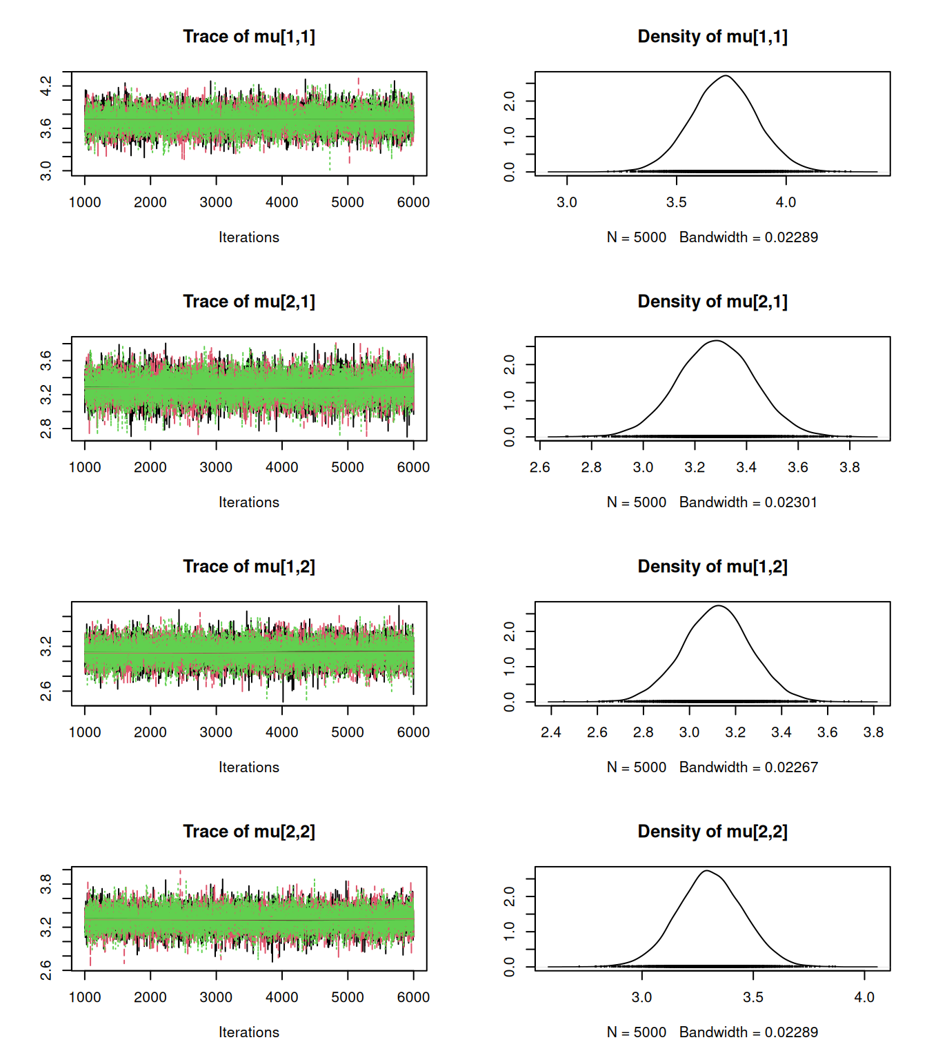
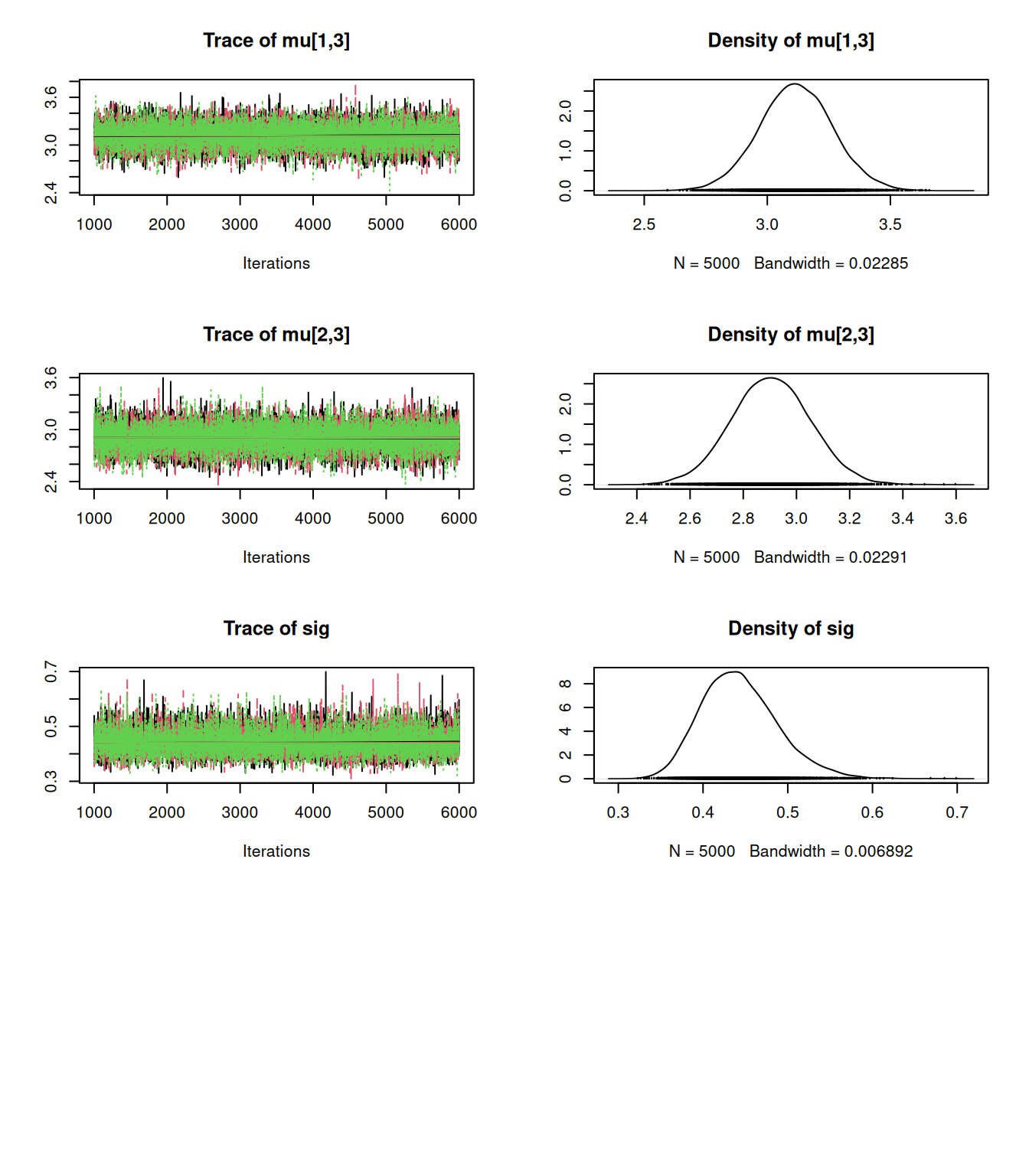
## convergence diagnostics
gelman.diag(mod3_sim)
Potential scale reduction factors:
Point est. Upper C.I.
mu[1,1] 1 1
mu[2,1] 1 1
mu[1,2] 1 1
mu[2,2] 1 1
mu[1,3] 1 1
mu[2,3] 1 1
sig 1 1
Multivariate psrf
1autocorr.diag(mod3_sim) mu[1,1] mu[2,1] mu[1,2] mu[2,2] mu[1,3]
Lag 0 1.000000000 1.000000000 1.000000000 1.0000000000 1.000000000
Lag 1 -0.005018705 0.008152441 0.015313498 0.0029797885 0.004469142
Lag 5 0.016177408 -0.021799649 0.010400377 -0.0008634916 -0.014815307
Lag 10 -0.009514649 0.004054763 -0.004133183 0.0078824679 -0.006126892
Lag 50 0.001873124 0.011662140 0.002653627 -0.0148359827 0.002095702
mu[2,3] sig
Lag 0 1.000000000 1.000000000
Lag 1 -0.011307532 0.117368828
Lag 5 0.001201311 -0.004591564
Lag 10 -0.012132645 0.021469777
Lag 50 -0.012255574 -0.002188778effectiveSize(mod3_sim) mu[1,1] mu[2,1] mu[1,2] mu[2,2] mu[1,3] mu[2,3] sig
15000.00 15000.00 14720.04 15451.89 14799.45 15212.59 11675.97 raftery.diag(mod3_sim)[[1]]
Quantile (q) = 0.025
Accuracy (r) = +/- 0.005
Probability (s) = 0.95
Burn-in Total Lower bound Dependence
(M) (N) (Nmin) factor (I)
mu[1,1] 2 3866 3746 1.030
mu[2,1] 3 4062 3746 1.080
mu[1,2] 2 3995 3746 1.070
mu[2,2] 2 3995 3746 1.070
mu[1,3] 2 3866 3746 1.030
mu[2,3] 2 3680 3746 0.982
sig 2 3866 3746 1.030
[[2]]
Quantile (q) = 0.025
Accuracy (r) = +/- 0.005
Probability (s) = 0.95
Burn-in Total Lower bound Dependence
(M) (N) (Nmin) factor (I)
mu[1,1] 2 3741 3746 0.999
mu[2,1] 2 3741 3746 0.999
mu[1,2] 2 3741 3746 0.999
mu[2,2] 2 3866 3746 1.030
mu[1,3] 2 3995 3746 1.070
mu[2,3] 2 3680 3746 0.982
sig 2 3803 3746 1.020
[[3]]
Quantile (q) = 0.025
Accuracy (r) = +/- 0.005
Probability (s) = 0.95
Burn-in Total Lower bound Dependence
(M) (N) (Nmin) factor (I)
mu[1,1] 2 3741 3746 0.999
mu[2,1] 2 3741 3746 0.999
mu[1,2] 2 3741 3746 0.999
mu[2,2] 2 3803 3746 1.020
mu[1,3] 2 3995 3746 1.070
mu[2,3] 2 3866 3746 1.030
sig 2 3930 3746 1.050 Let’s compute the DIC and compare with our previous models.
(dic3 = dic.samples(mod3, n.iter=1e3))Mean deviance: 52.15
penalty 7.282
Penalized deviance: 59.43 dic2Mean deviance: 55.61
penalty 5.213
Penalized deviance: 60.83 dic1Mean deviance: 66.64
penalty 3.997
Penalized deviance: 70.64 This suggests that the full model with interaction between wool and tension (which is equivalent to the cell means model) is the best for explaining/predicting warp breaks.
summary(mod3_sim)
Iterations = 1001:6000
Thinning interval = 1
Number of chains = 3
Sample size per chain = 5000

1. Empirical mean and standard deviation for each variable,
   plus standard error of the mean:

          Mean      SD  Naive SE Time-series SE
mu[1,1] 3.7190 0.14825 0.0012105      0.0012102
mu[2,1] 3.2805 0.14895 0.0012162      0.0012163
mu[1,2] 3.1149 0.15169 0.0012386      0.0012510
mu[2,2] 3.3081 0.15015 0.0012260      0.0012091
mu[1,3] 3.1213 0.14902 0.0012167      0.0012252
mu[2,3] 2.9039 0.14927 0.0012188      0.0012105
sig     0.4437 0.04488 0.0003664      0.0004155

2. Quantiles for each variable:

          2.5%    25%    50%    75%  97.5%
mu[1,1] 3.4272 3.6201 3.7190 3.8171 4.0131
mu[2,1] 2.9854 3.1829 3.2815 3.3782 3.5734
mu[1,2] 2.8161 3.0139 3.1146 3.2155 3.4128
mu[2,2] 3.0111 3.2086 3.3087 3.4080 3.6012
mu[1,3] 2.8325 3.0202 3.1204 3.2211 3.4144
mu[2,3] 2.6075 2.8054 2.9048 3.0038 3.1949
sig 0.3668 0.4123 0.4396 0.4708 0.5433HPDinterval(mod3_csim) lower upper
mu[1,1] 3.4367959 4.0199878
mu[2,1] 2.9798602 3.5668917
mu[1,2] 2.8067009 3.3994604
mu[2,2] 3.0154010 3.6040241
mu[1,3] 2.8261102 3.4051581
mu[2,3] 2.6166368 3.2013581
sig 0.3625479 0.5352691
attr(,"Probability")
[1] 0.95par(mfrow=c(3,2)) # arrange frame for plots
densplot(mod3_csim[,1:6], xlim=c(2.0, 4.5))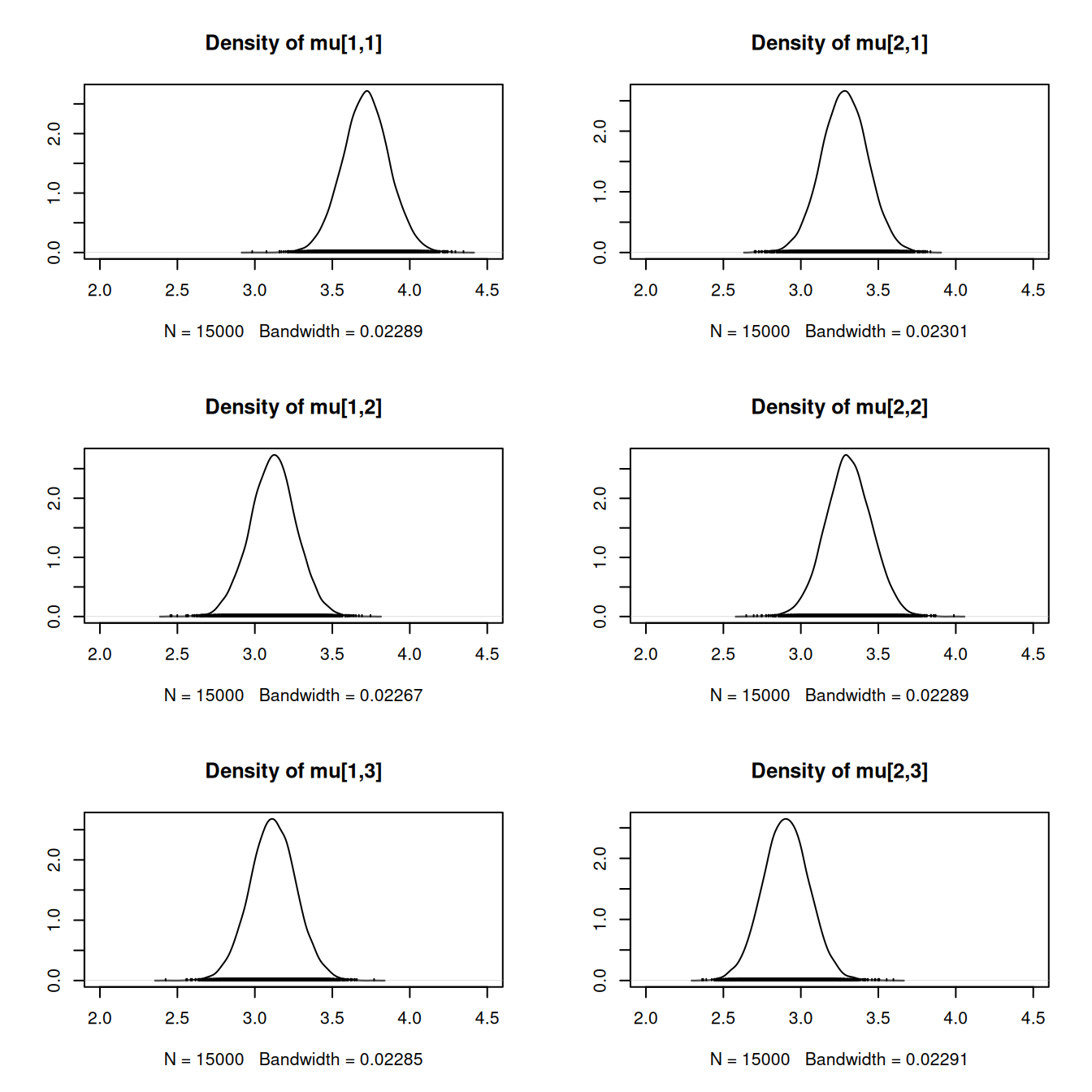
It might be tempting to look at comparisons between each combination of treatments, but we warn that this could yield spurious results. When we discussed the statistical modeling cycle, we said it is best not to search your results for interesting hypotheses, because if there are many hypotheses, some will appear to show “effects” or “associations” simply due to chance. Results are most reliable when we determine a relatively small number of hypotheses we are interested in beforehand, collect the data, and statistically evaluate the evidence for them.
One question we might be interested in with these data is finding the treatment combination that produces the fewest breaks. To calculate this, we can go through our posterior samples and for each sample, find out which group has the smallest mean. These counts help us determine the posterior probability that each of the treatment groups has the smallest mean.
prop.table( table( apply(mod3_csim[,1:6], 1, which.min) ) )
         2          3          4          5          6
0.01680000 0.12126667 0.01193333 0.11113333 0.73886667
The evidence supports wool B with high tension as the treatment that produces the fewest breaks.