151 L06 : Proof of Lemmas 1-3 for the outer-measure extension construction

Video 151.1: Lesson 6: Proof of Lemmas 1–3 for the outer-measure extension construction.

151.1 Lesson map

This lesson proves the first three lemmas from the extension roadmap.

• 0:12 — Recap: extending P from a field \mathcal{F}_0 to \mathcal{F}=\sigma(\mathcal{F}_0).
• 2:50 — Recall the outer measure P^*.
• 4:18 — Important warning: do not use that P^* is a probability measure yet.
• 4:36 — Recall the definition of \mathcal{M}.
• 6:31 — Lemma 1: \mathcal{M} is a field.
• 17:54 — Lemma 2: P^* is countably additive on disjoint sets in \mathcal{M}.
• 26:41 — Lemma 3: \mathcal{M} is a \sigma-field.

151.2 Recap: the extension problem

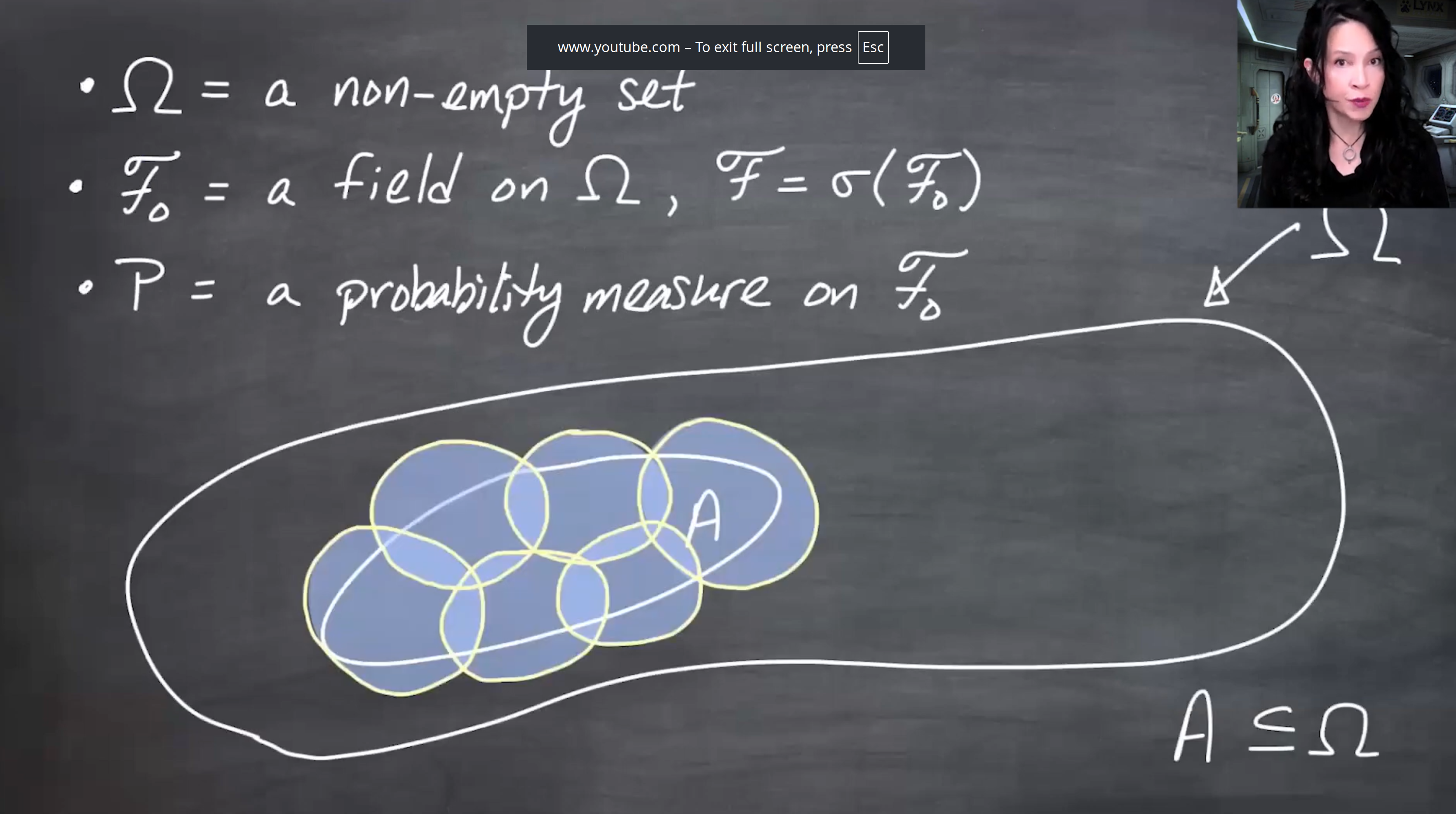
We start with a non-empty set \Omega, a field \mathcal{F}_0 on \Omega, and a probability measure

P:\mathcal{F}_0\to[0,1].

Let

\mathcal{F}=\sigma(\mathcal{F}_0)

be the \sigma-field generated by \mathcal{F}_0.

The goal is to extend P to a probability measure on \mathcal{F}, while preserving the old values:

P^*(A)=P(A) \qquad \text{for all } A\in\mathcal{F}_0.

Extending a probability measure from a field to a generated sigma-field.

Figure 151.1: The extension problem starts from P on the smaller field \mathcal{F}_0 and aims to define a probability measure on the larger \sigma-field \mathcal{F}=\sigma(\mathcal{F}_0).

The previous lesson gave the roadmap using six lemmas. This lesson proves Lemmas 1–3.

The six-lemma roadmap, with this lesson focused on Lemmas 1 through 3.

Figure 151.2: The proof is optional in the sense that the previous lesson already showed how the lemmas imply the extension theorem. This lesson supplies the missing proof details.

151.3 Recall the outer measure P^*

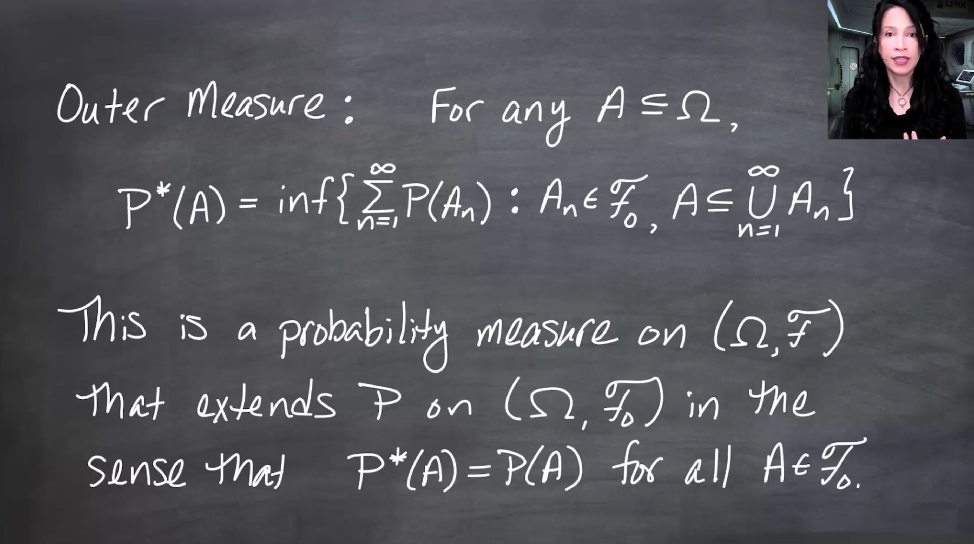
For every subset A\subseteq\Omega, define

P^*(A) = \inf \left\{ \sum_{n=1}^{\infty}P(A_n) : A_n\in\mathcal{F}_0 \text{ and } A\subseteq\bigcup_{n=1}^{\infty}A_n \right\}.

This measures A from the outside by covering it with countably many sets from \mathcal{F}_0.

Definition of P star as an infimum over cover sums.

Figure 151.3: The sets A_n come from \mathcal{F}_0, where P is already defined. The infimum searches over all such covers and chooses the best upper estimate.

P star is not yet available as a probability measure during the lemma proofs.

Figure 151.4: During these proofs, we may use the already-proved basic properties of P^*, such as P^*(\emptyset)=0, monotonicity, and countable subadditivity. We may not use countable additivity of P^* as if it were already a probability measure.

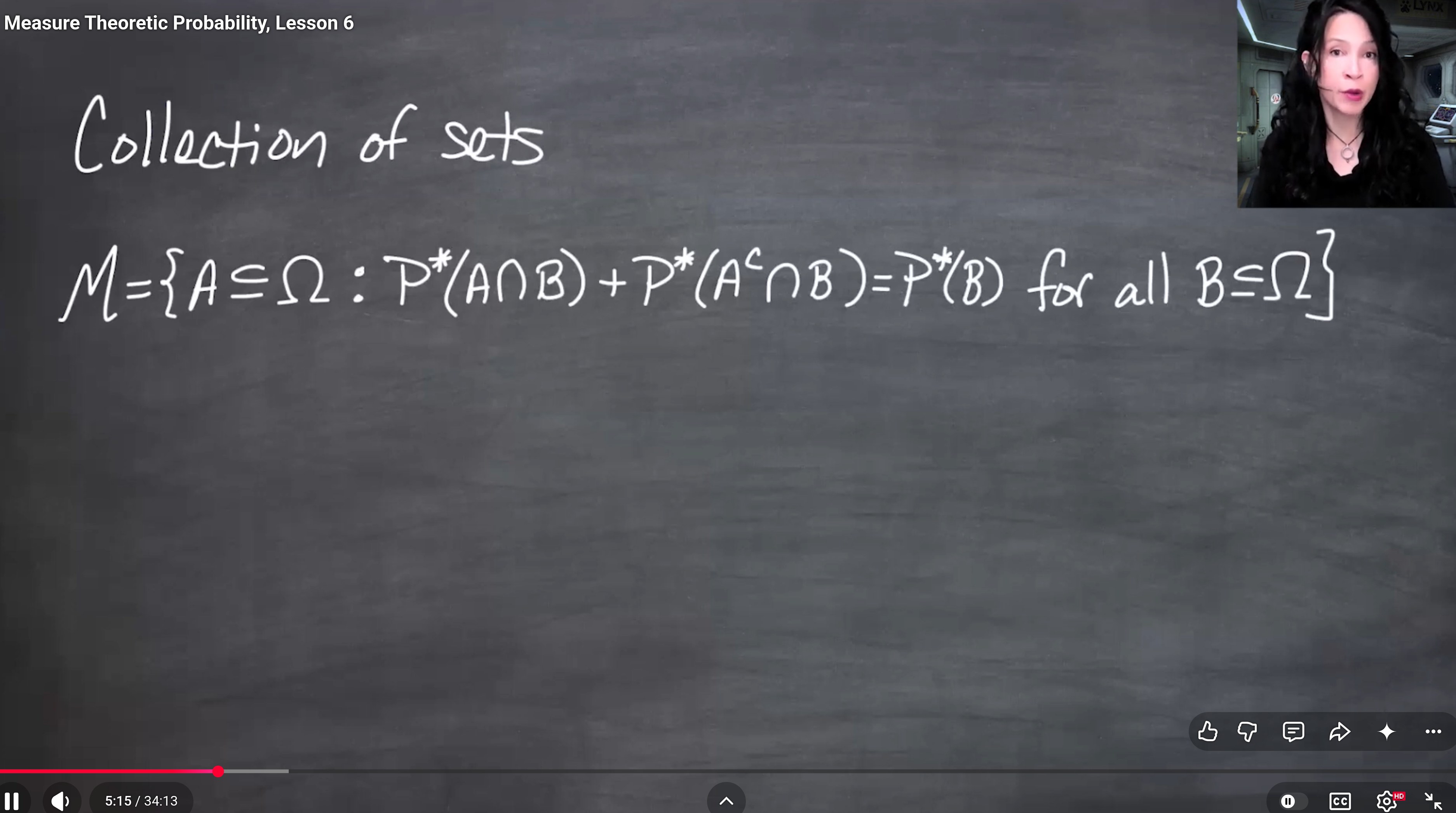
151.4 Recall the class \mathcal{M}

Define \mathcal{M} as the class of subsets A\subseteq\Omega that split every subset B\subseteq\Omega additively:

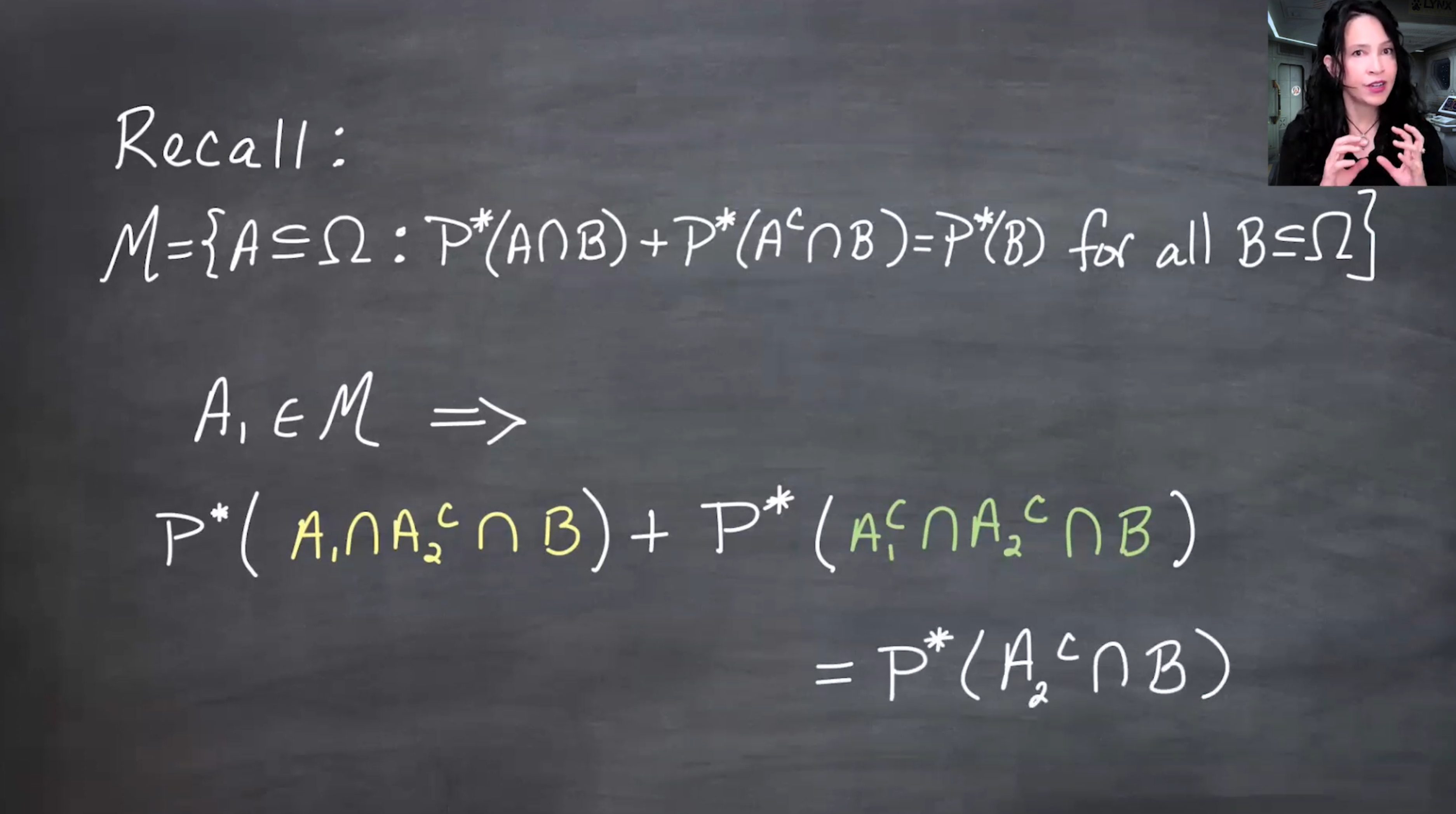
\mathcal{M} = \left\{ A\subseteq\Omega: P^*(A\cap B)+P^*(A^c\cap B)=P^*(B) \text{ for all } B\subseteq\Omega \right\}.

Definition of the class M.

Figure 151.5: The sets in \mathcal{M} are the sets that behave measurably with respect to the outer measure P^*: they cut every B into two pieces without losing or gaining P^*-mass.

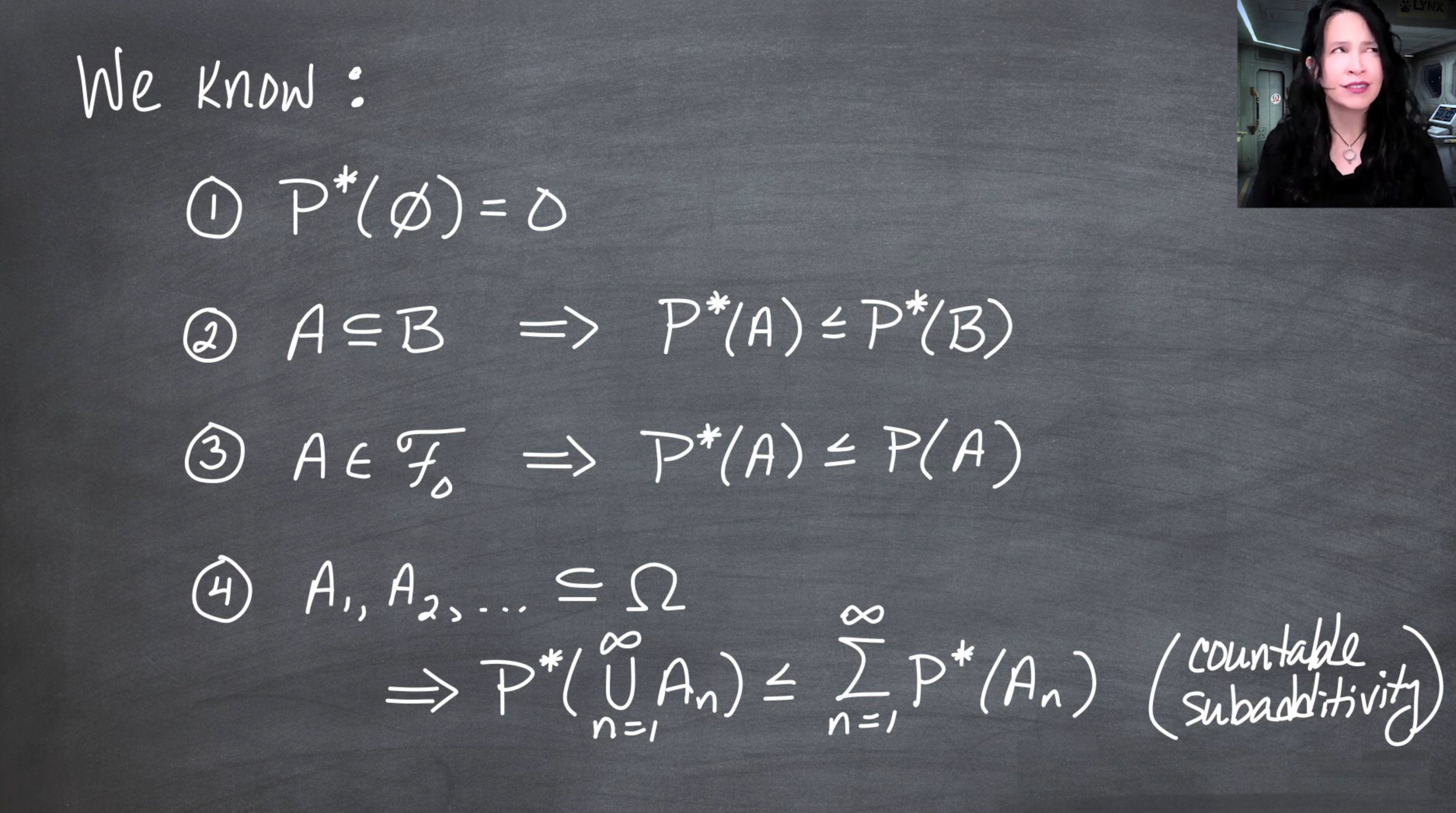
Because P^* is countably subadditive, we always have

P^*(B) \leq P^*(A\cap B)+P^*(A^c\cap B).

So to show A\in\mathcal{M}, it is enough to prove the reverse inequality:

P^*(A\cap B)+P^*(A^c\cap B) \leq P^*(B) \qquad \text{for all } B\subseteq\Omega.

Equivalent inequality criterion for membership in M.

Figure 151.6: The equality definition and the one-sided inequality criterion are equivalent because subadditivity already gives the other direction.

The sets in \mathcal{M} are sometimes called P^*-measurable sets.

The sets in M are called P star measurable sets.

Figure 151.7: The terminology “P^*-measurable” reflects the role of \mathcal{M}: it is the class on which P^* will become a genuine probability measure.

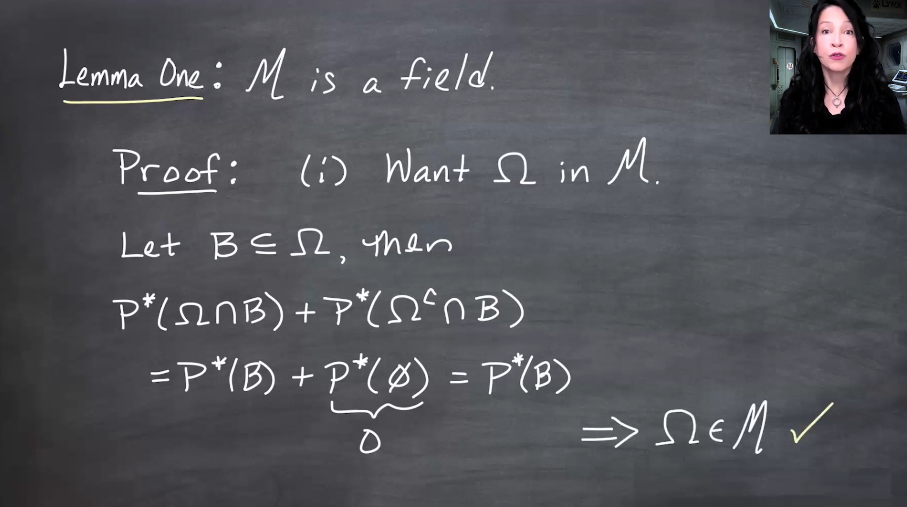
151.5 Lemma 1: \mathcal{M} is a field

Lemma 151.1 (Lemma 1) The collection \mathcal{M} is a field.

To prove this, show:

1. \Omega\in\mathcal{M};
2. if A\in\mathcal{M}, then A^c\in\mathcal{M};
3. if A_1,A_2\in\mathcal{M}, then A_1\cup A_2\in\mathcal{M}.

Finite unions then follow by induction.

Lemma 1 states that M is a field.

Figure 151.8: A field requires the full space, closure under complements, and closure under finite unions.

151.5.1 Step 1: \Omega\in\mathcal{M}

For any B\subseteq\Omega,

P^*(\Omega\cap B)+P^*(\Omega^c\cap B) = P^*(B)+P^*(\emptyset) = P^*(B).

Since P^*(\emptyset)=0, this proves \Omega\in\mathcal{M}.

Showing Omega belongs to M.

Figure 151.9: The full space splits any B into B and \emptyset, so the defining equality for \mathcal{M} holds.

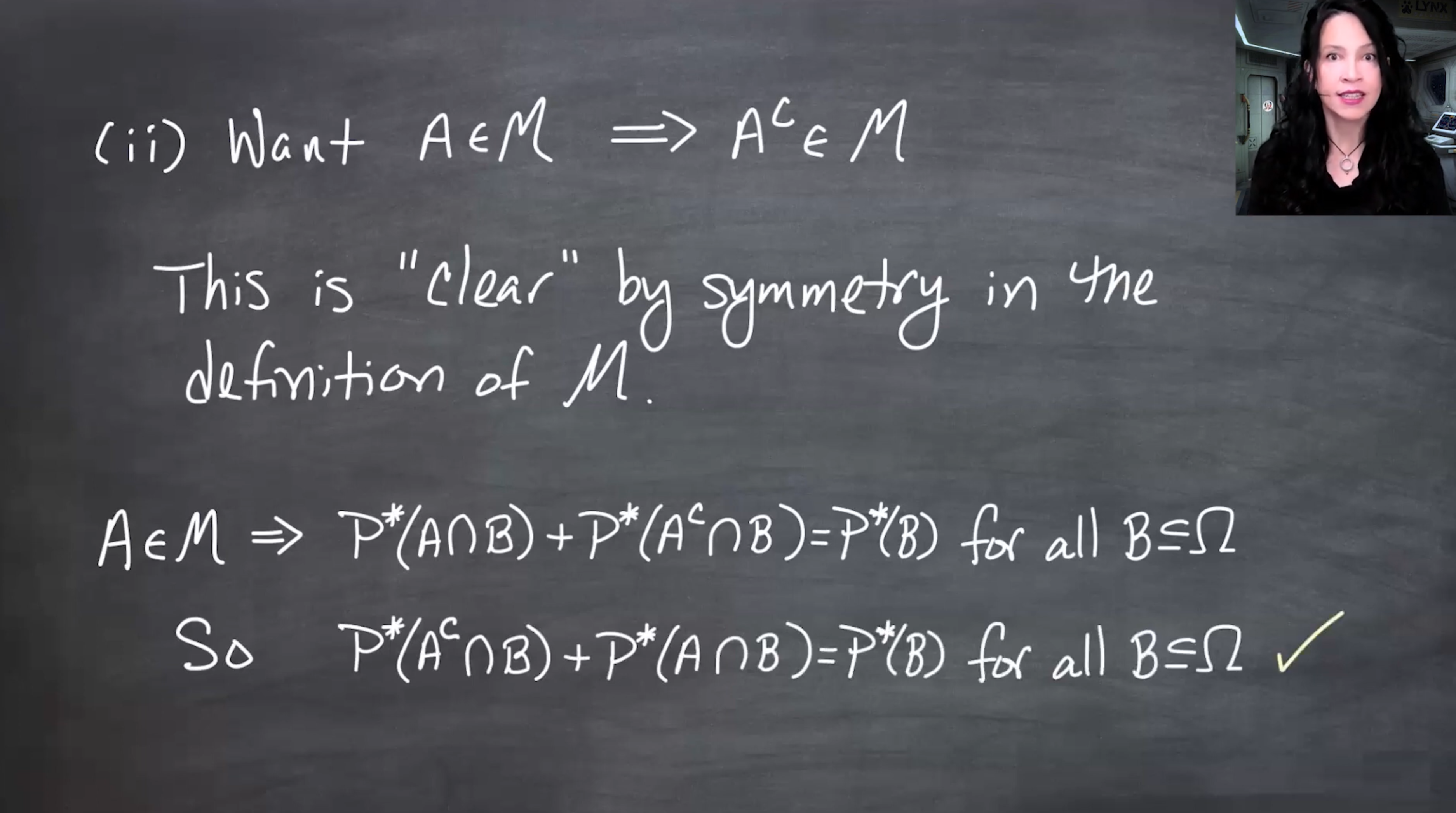
151.5.2 Step 2: closure under complements

If A\in\mathcal{M}, then for every B\subseteq\Omega,

P^*(A\cap B)+P^*(A^c\cap B) = P^*(B).

But the two summands can be swapped:

P^*(A^c\cap B)+P^*((A^c)^c\cap B) = P^*(B).

Thus A^c\in\mathcal{M}.

Closure of M under complements.

Figure 151.10: The definition of \mathcal{M} is symmetric in A and A^c, so complements are immediate.

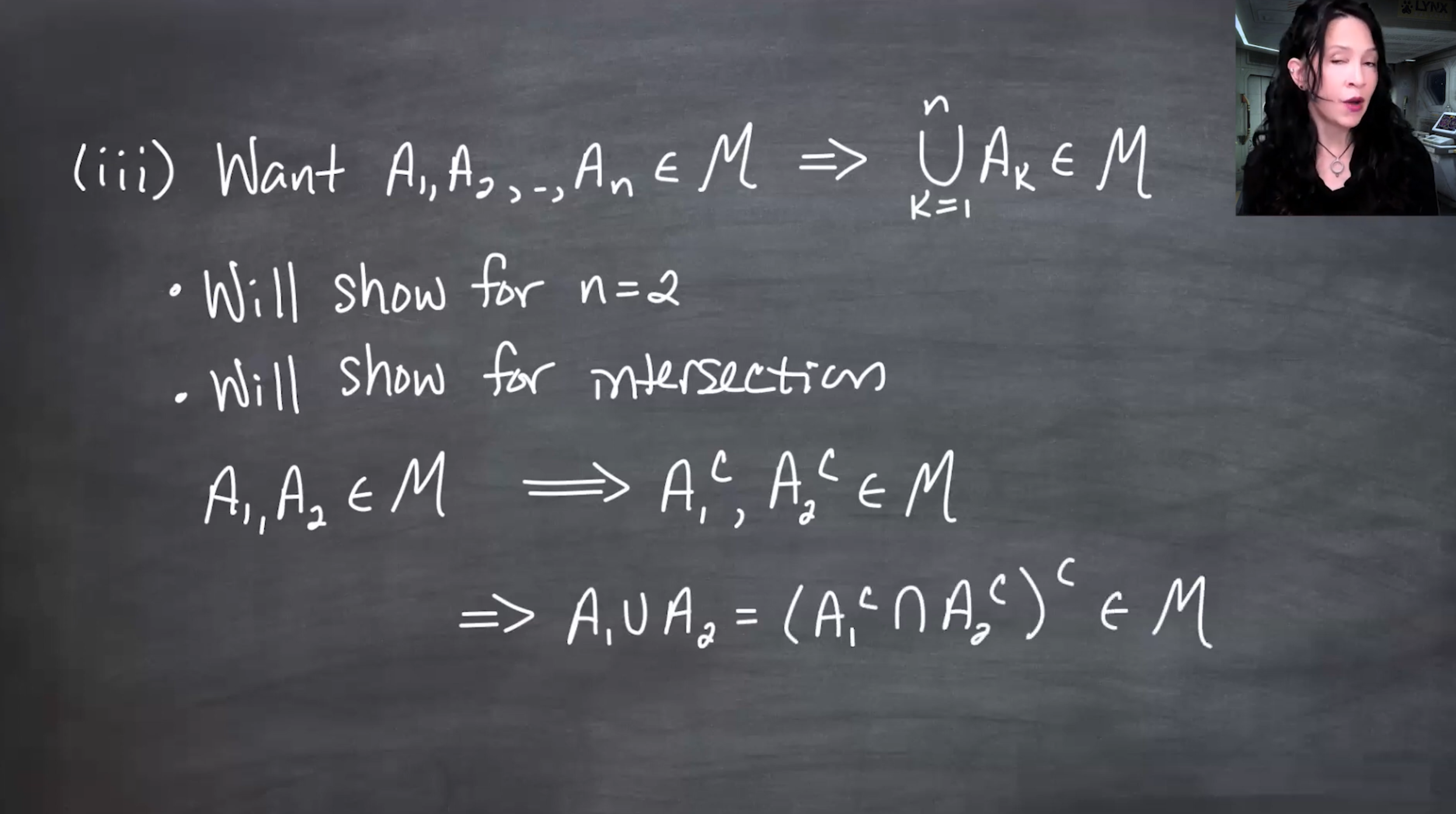
151.5.3 Step 3: closure under finite unions

It is easier to prove closure under finite intersections first. Then De Morgan’s law gives closure under finite unions.

If A_1,A_2\in\mathcal{M}, we will prove

A_1\cap A_2\in\mathcal{M}.

Then

A_1\cup A_2 = (A_1^c\cap A_2^c)^c

belongs to \mathcal{M} because \mathcal{M} is closed under complements and finite intersections.

Using intersections and De Morgan’s law to prove finite union closure.

Figure 151.11: The proof uses the identity A_1\cup A_2=(A_1^c\cap A_2^c)^c. So it is enough to prove closure under intersections.

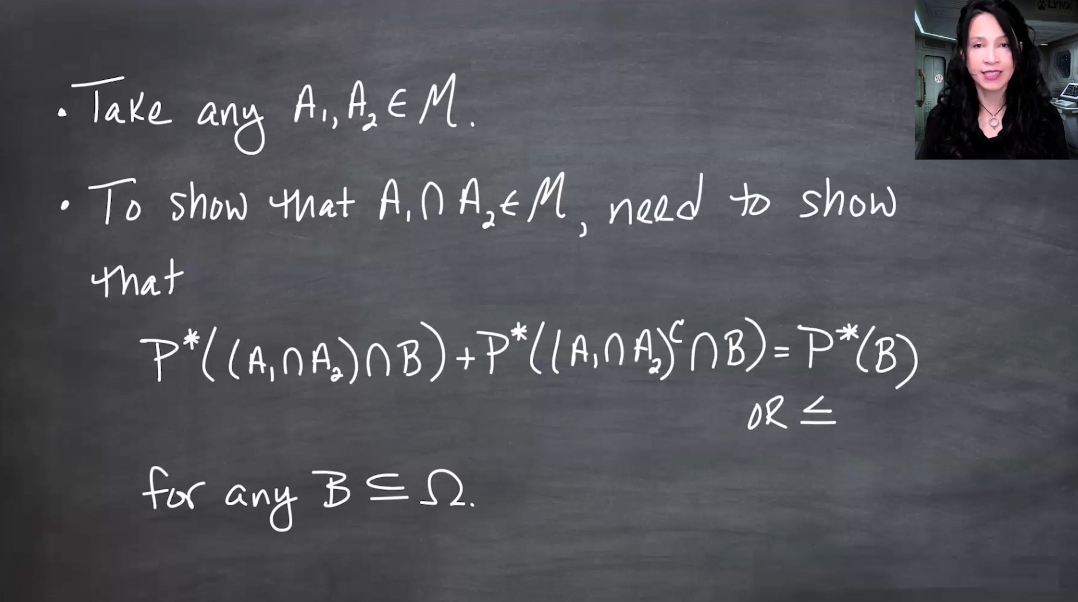
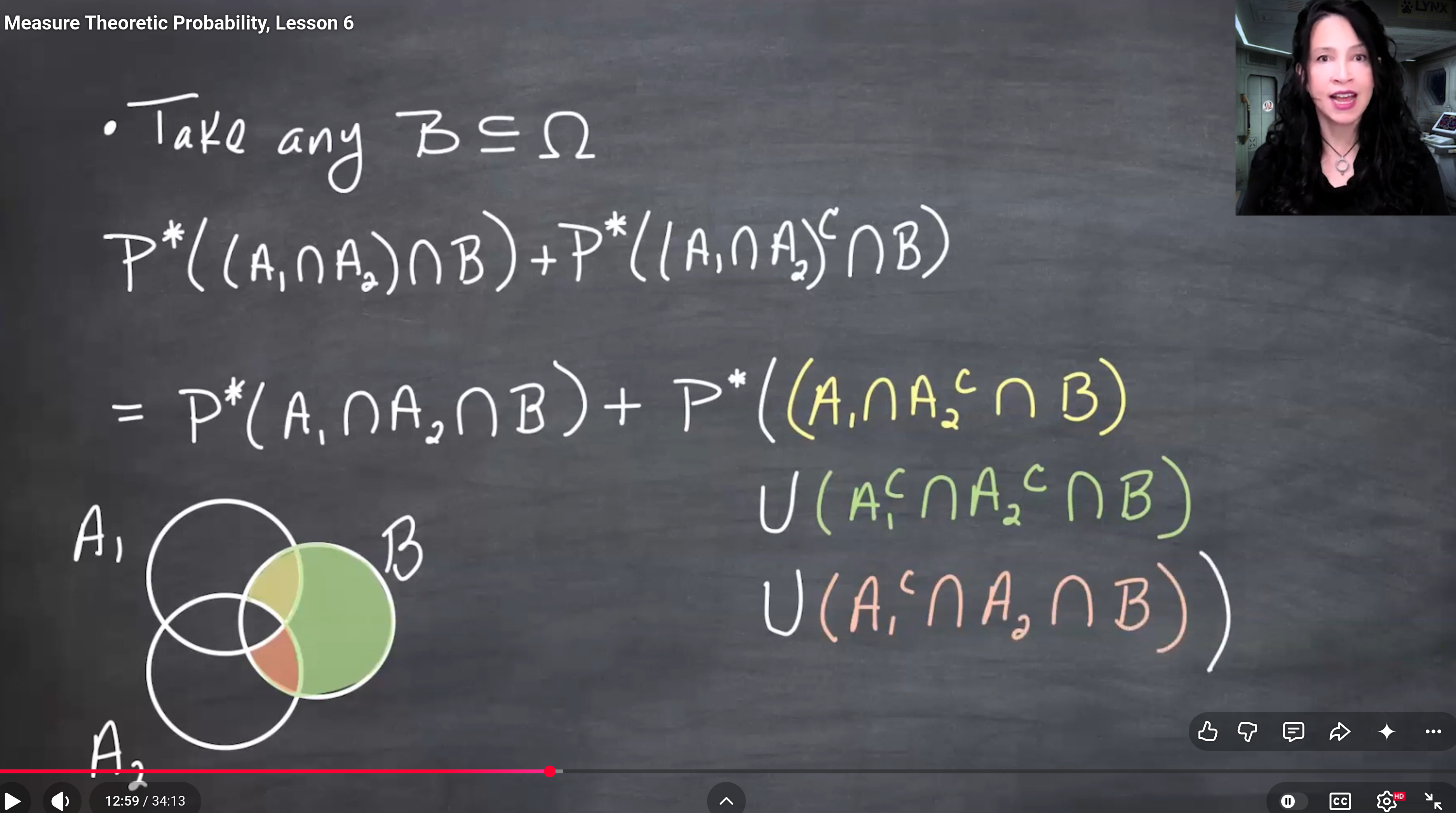
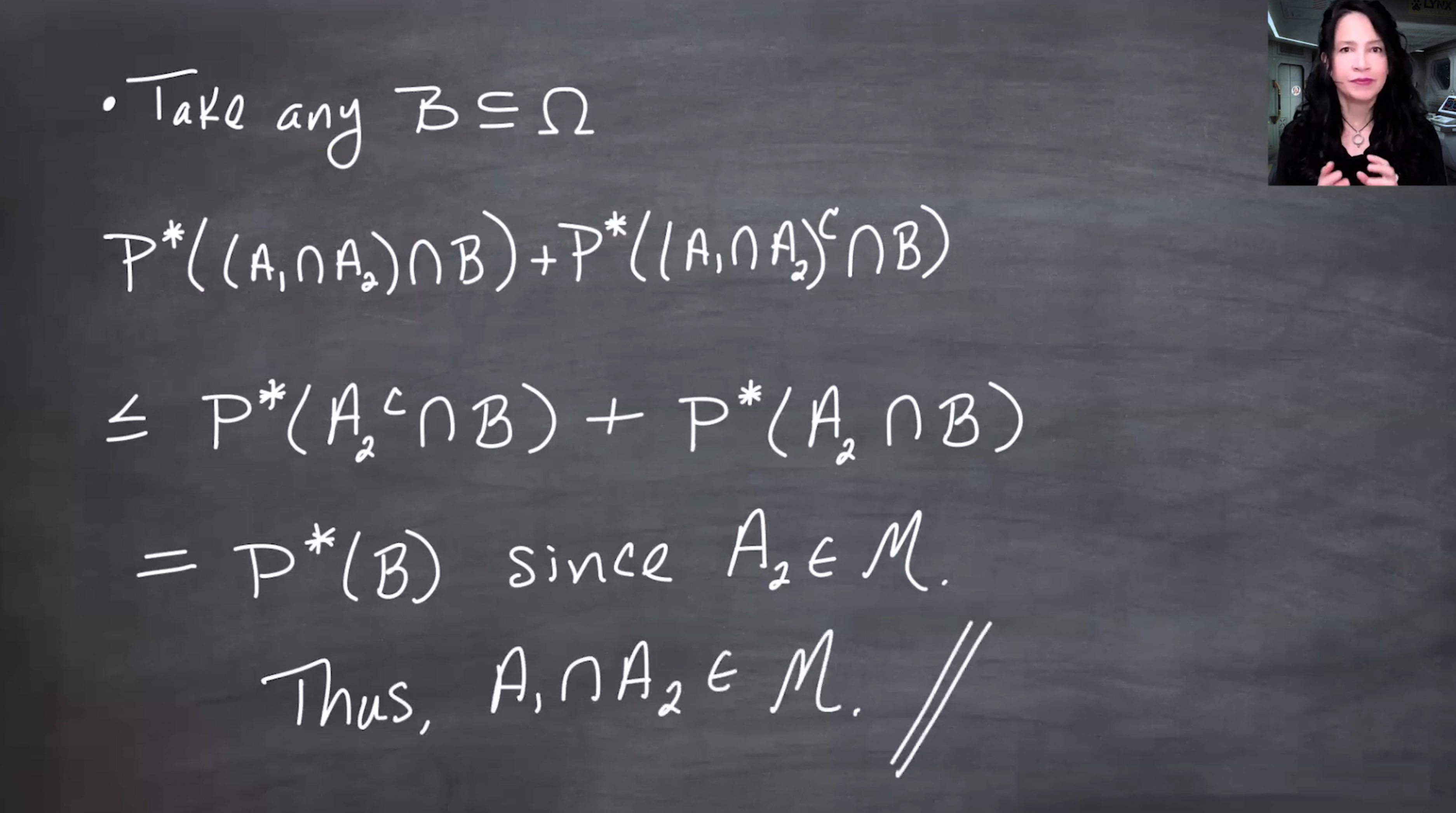
To show A_1\cap A_2\in\mathcal{M}, take any B\subseteq\Omega. We need to show

P^*((A_1\cap A_2)\cap B) + P^*((A_1\cap A_2)^c\cap B) \leq P^*(B).

The second set is the part of B outside A_1\cap A_2.

Beginning the proof that intersections of M sets are in M.

Figure 151.12: The proof uses the one-sided criterion for membership in \mathcal{M}, because the reverse inequality is already supplied by subadditivity.

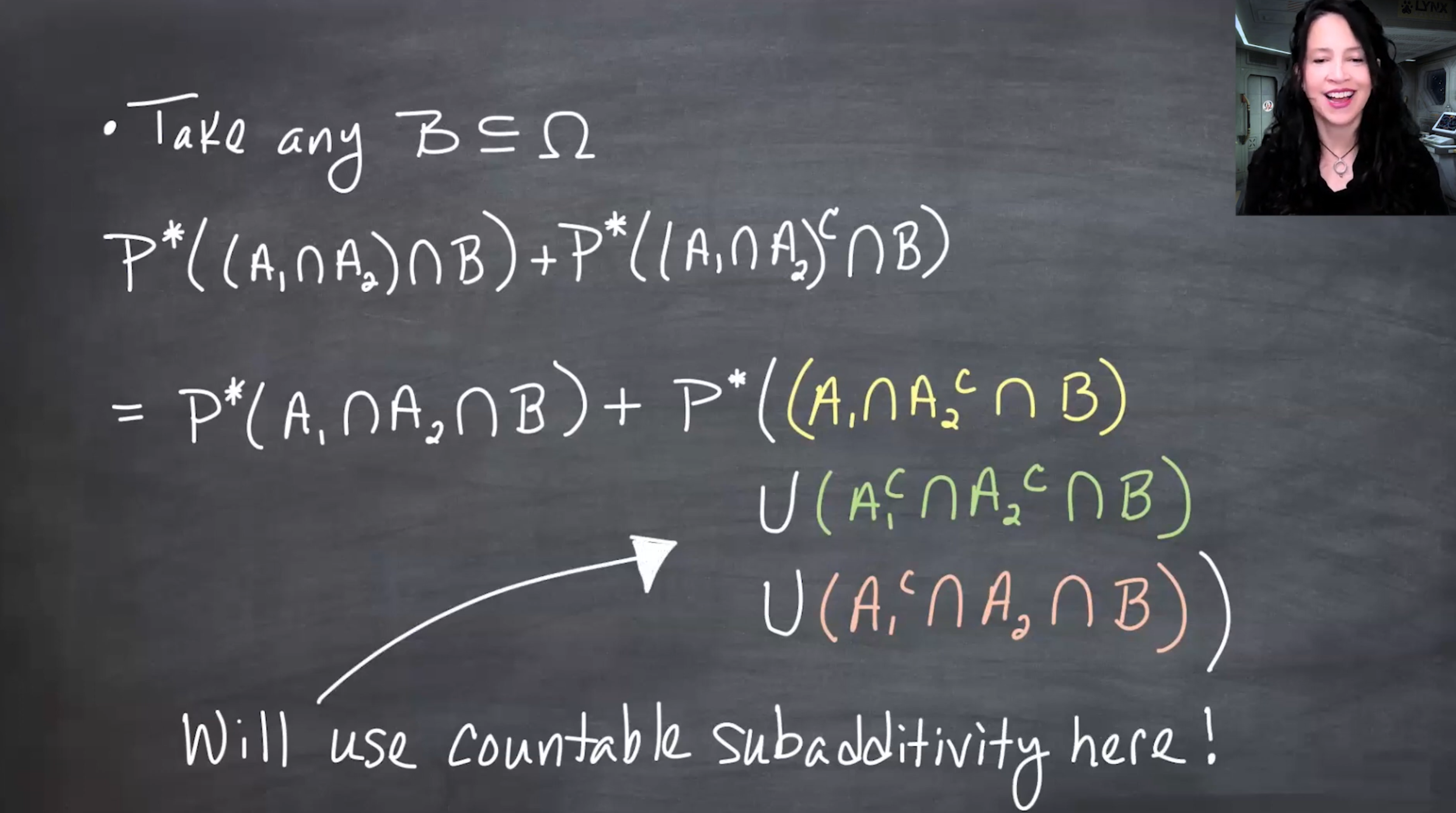
The set outside A_1\cap A_2 but inside B can be decomposed into three regions:

(A_1\cap A_2)^c\cap B = (A_1\cap A_2^c\cap B) \cup (A_1^c\cap A_2^c\cap B) \cup (A_1^c\cap A_2\cap B).

Decomposing the part of B outside A1 intersect A2.

Figure 151.13: The Venn diagram splits B\setminus(A_1\cap A_2) into the pieces where only A_1 holds, neither holds, or only A_2 holds.

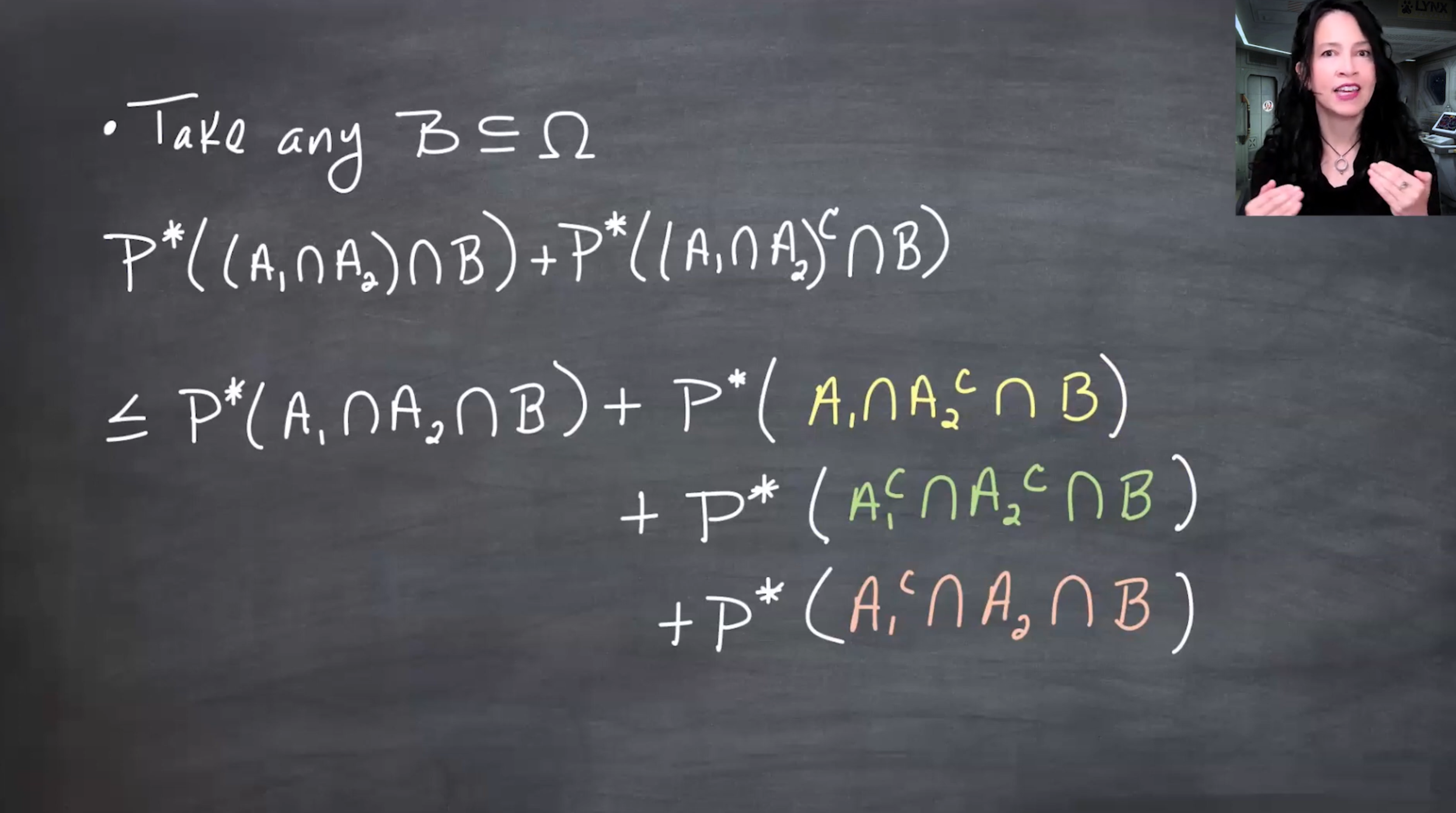
By countable subadditivity of P^*, the P^* of this union is bounded above by the sum of the three P^* values.

Using subadditivity to bound the decomposed union.

Figure 151.14: This is one of the places where the proof must use subadditivity, not additivity, because P^* has not yet been proved to be a measure.

Now group the terms using the defining property of A_1\in\mathcal{M}.

For example,

P^*(A_1\cap A_2^c\cap B) + P^*(A_1^c\cap A_2^c\cap B) = P^*(A_2^c\cap B),

because this is the \mathcal{M} splitting property for A_1 applied to the test set A_2^c\cap B.

Combining terms using A1 in M.

Figure 151.15: The definition of \mathcal{M} lets us combine terms of the form P^*(A_1\cap C)+P^*(A_1^c\cap C) into P^*(C).

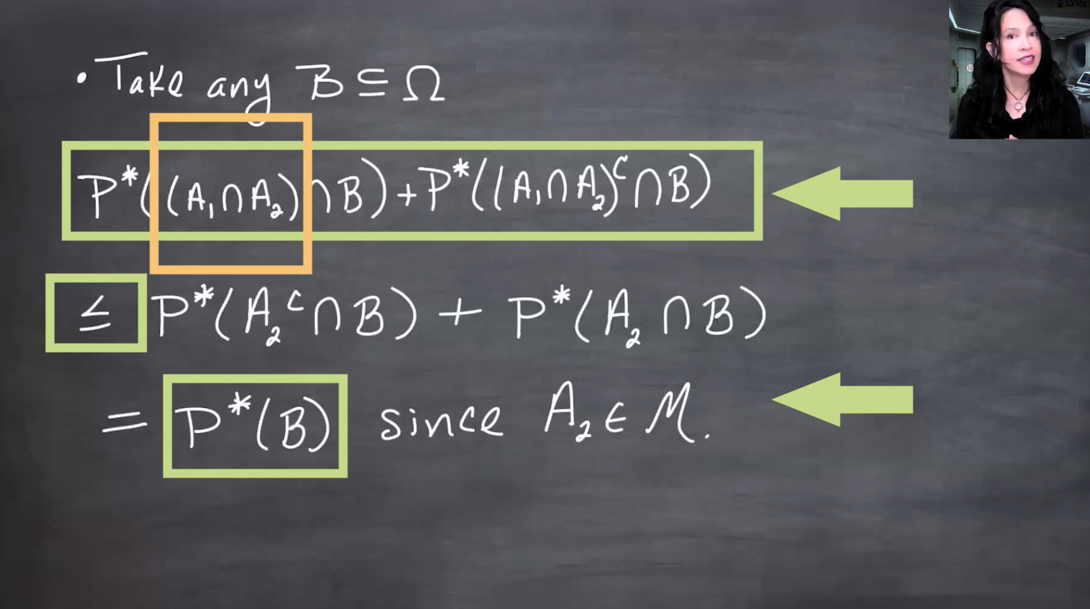
After grouping, the expression becomes

P^*(A_2\cap B)+P^*(A_2^c\cap B).

Since A_2\in\mathcal{M}, this equals P^*(B).

Using A2 in M to finish intersection closure.

Figure 151.16: The final step uses A_2\in\mathcal{M}. This proves A_1\cap A_2\in\mathcal{M}, and hence finite union closure follows by complements and De Morgan’s law.

Finite union closure for more than two sets follows by induction: once the union of two \mathcal{M}-sets is in \mathcal{M}, repeatedly union one more set.

Finite union closure follows by induction.

Figure 151.17: The proof for two sets is the essential case. The general finite case is repeated application of the two-set result.

Thus Lemma 1 is proved: \mathcal{M} is a field.

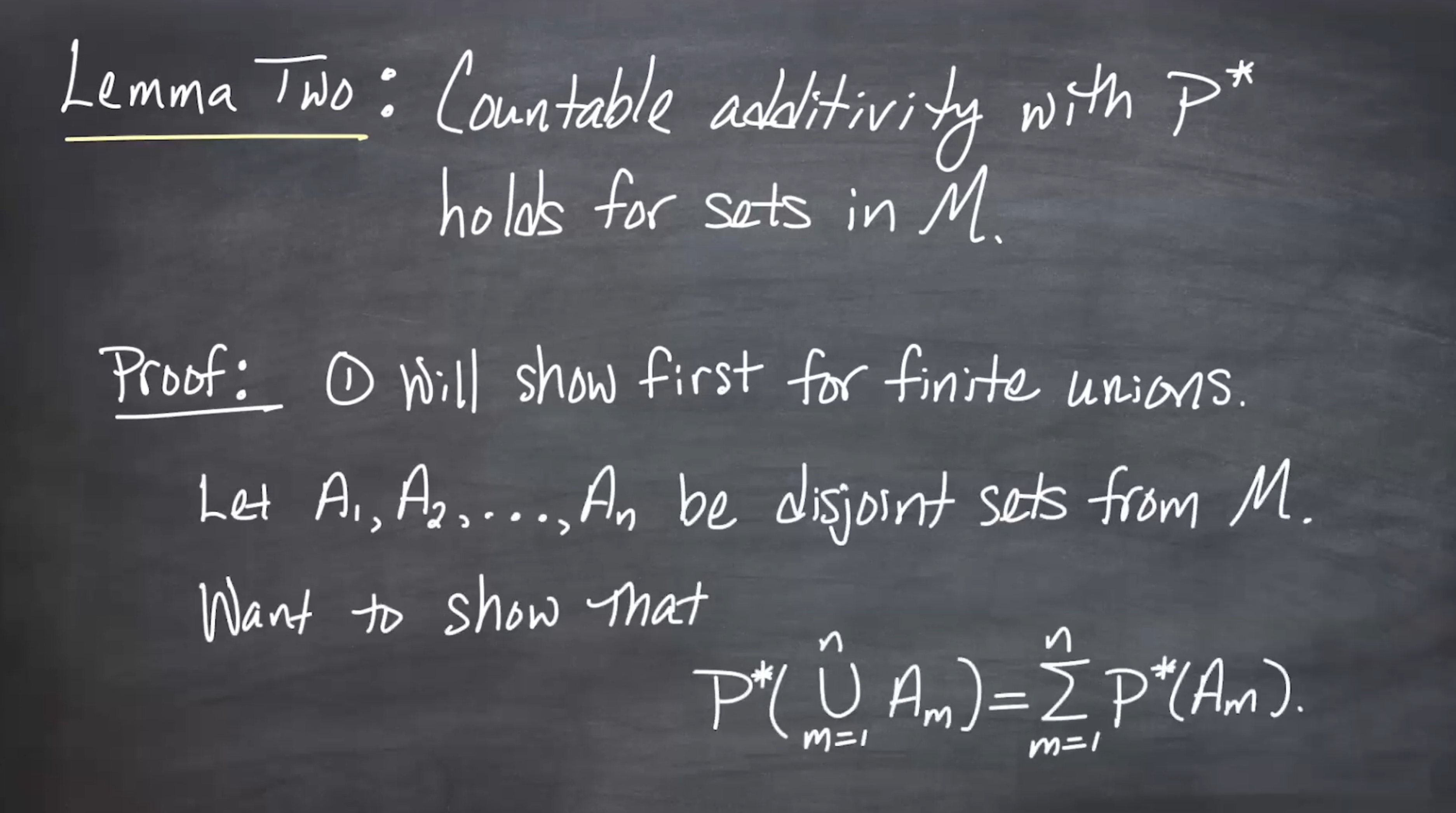
151.6 Lemma 2: countable additivity on \mathcal{M}

Lemma 151.2 (Lemma 2) If A_1,A_2,\ldots\in\mathcal{M} are disjoint, then

P^*\left(\bigcup_{n=1}^{\infty}A_n\right) = \sum_{n=1}^{\infty}P^*(A_n).

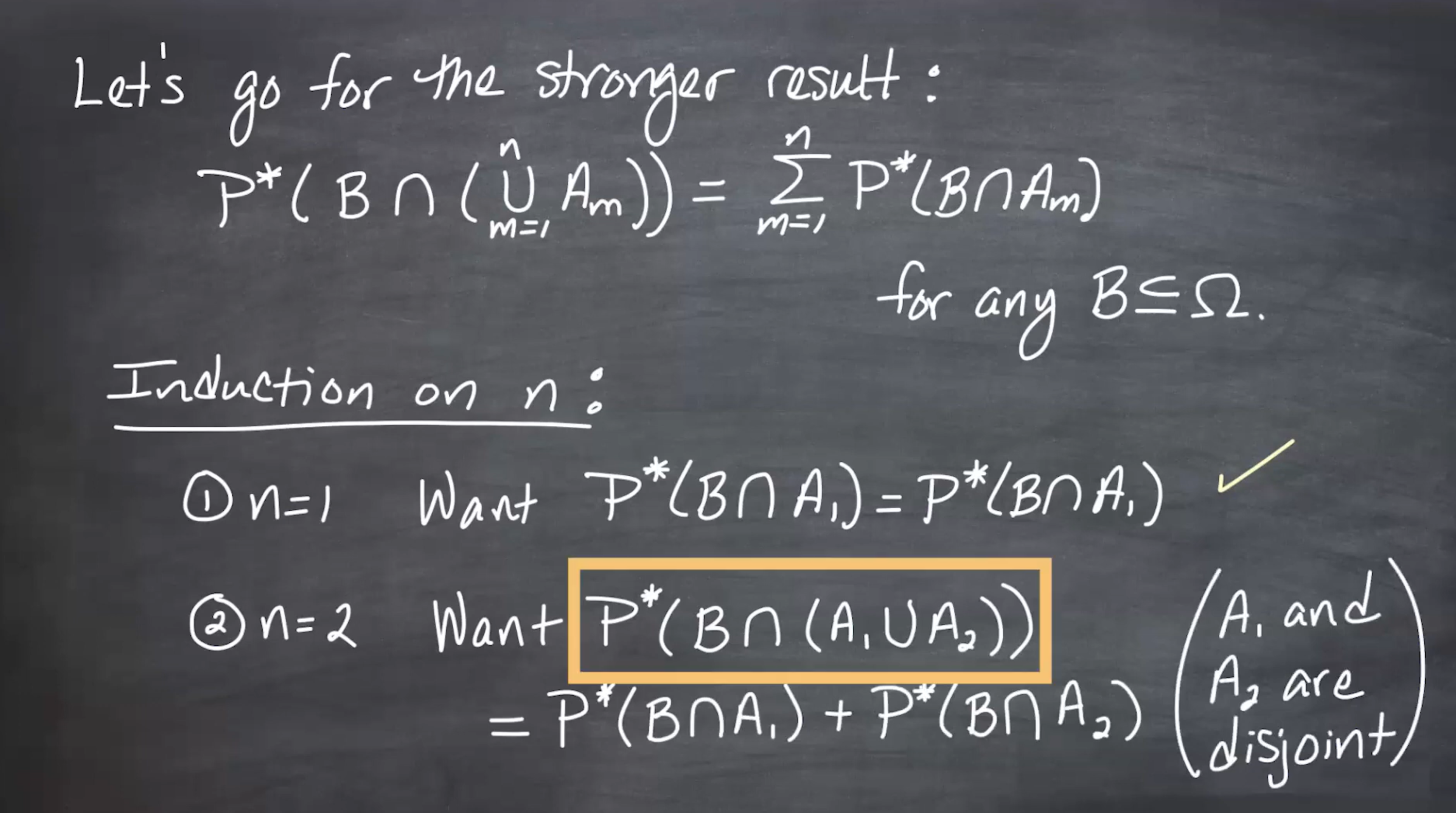
The proof first establishes a stronger finite version involving an arbitrary test set B\subseteq\Omega:

P^*\left(B\cap\bigcup_{i=1}^{n}A_i\right) = \sum_{i=1}^{n}P^*(B\cap A_i),

for disjoint A_1,\ldots,A_n\in\mathcal{M}.

Lemma 2 begins with finite additivity and a stronger statement involving B.

Figure 151.18: The stronger result includes a free subset B. Taking B=\Omega later recovers finite additivity for the A_i themselves.

151.6.1 Finite case

For n=1, the identity is trivial.

For n=2, take disjoint A_1,A_2\in\mathcal{M}. Then

B\cap(A_1\cup A_2)

splits into the part inside A_1 and the part inside A_2.

The n equals two finite case with a Venn diagram.

Figure 151.19: The diagram shows that B\cap(A_1\cup A_2) consists of two separated pieces: B\cap A_1 and B\cap A_2.

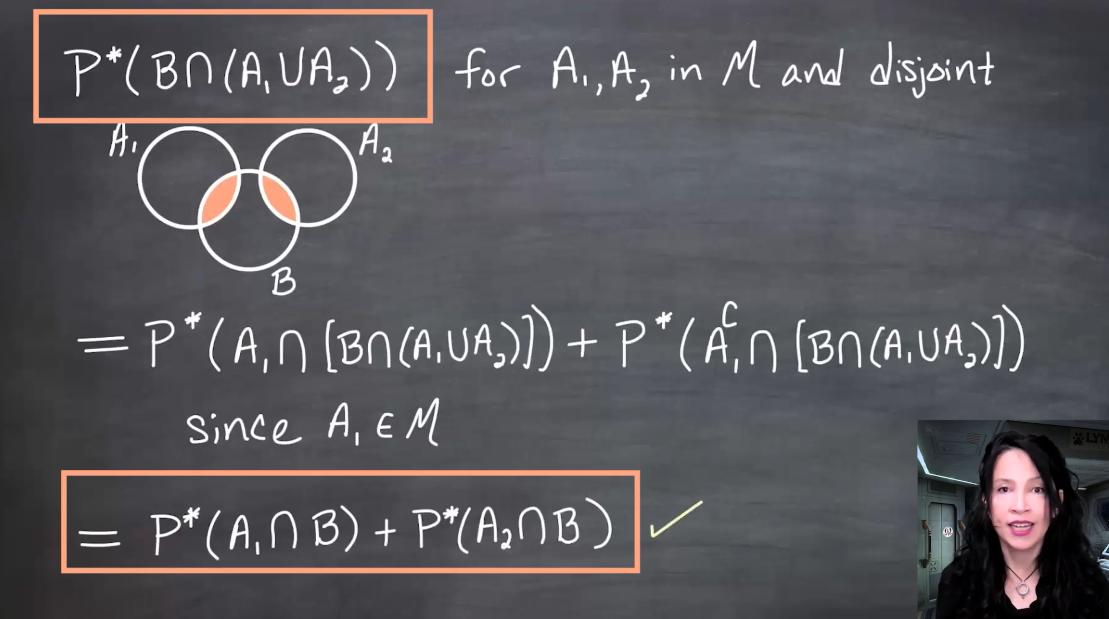
Using the defining property of A_1\in\mathcal{M}, applied to the test set B\cap(A_1\cup A_2),

P^*(B\cap(A_1\cup A_2)) = P^*(B\cap A_1)+P^*(B\cap A_2).

Using membership in M rather than assuming countable additivity.

Figure 151.20: This equality is not using countable additivity of P^*. It comes from the definition of membership in \mathcal{M}.

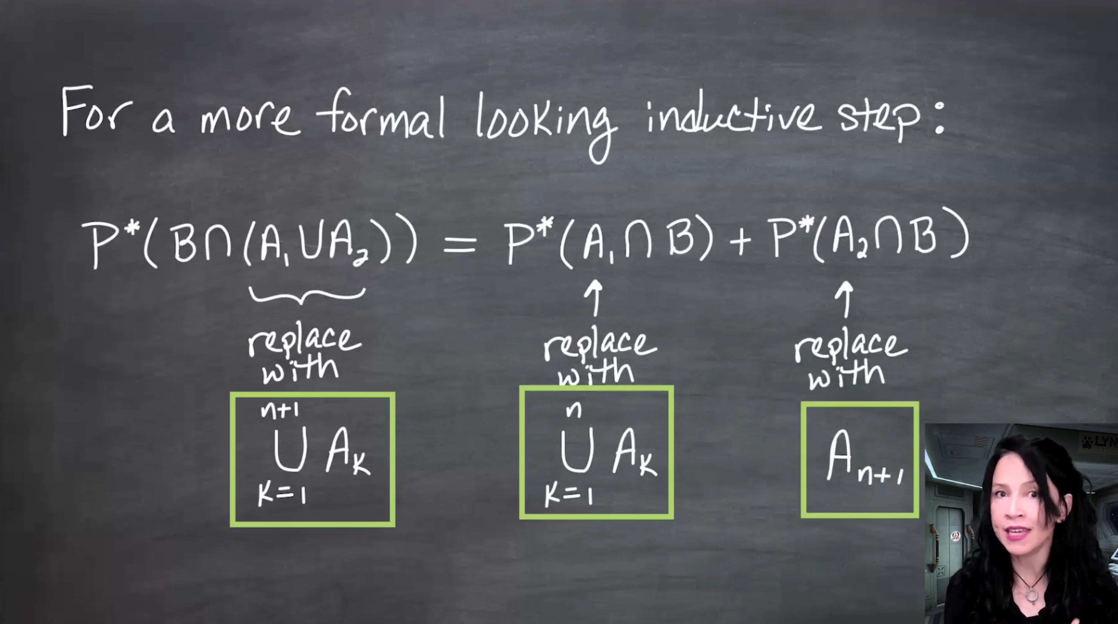
The finite case for general n follows by induction.

Induction extends the finite result to n disjoint sets.

Figure 151.21: To pass from n to n+1, treat \bigcup_{i=1}^n A_i as one \mathcal{M}-set and A_{n+1} as the second set.

151.6.2 Countable case

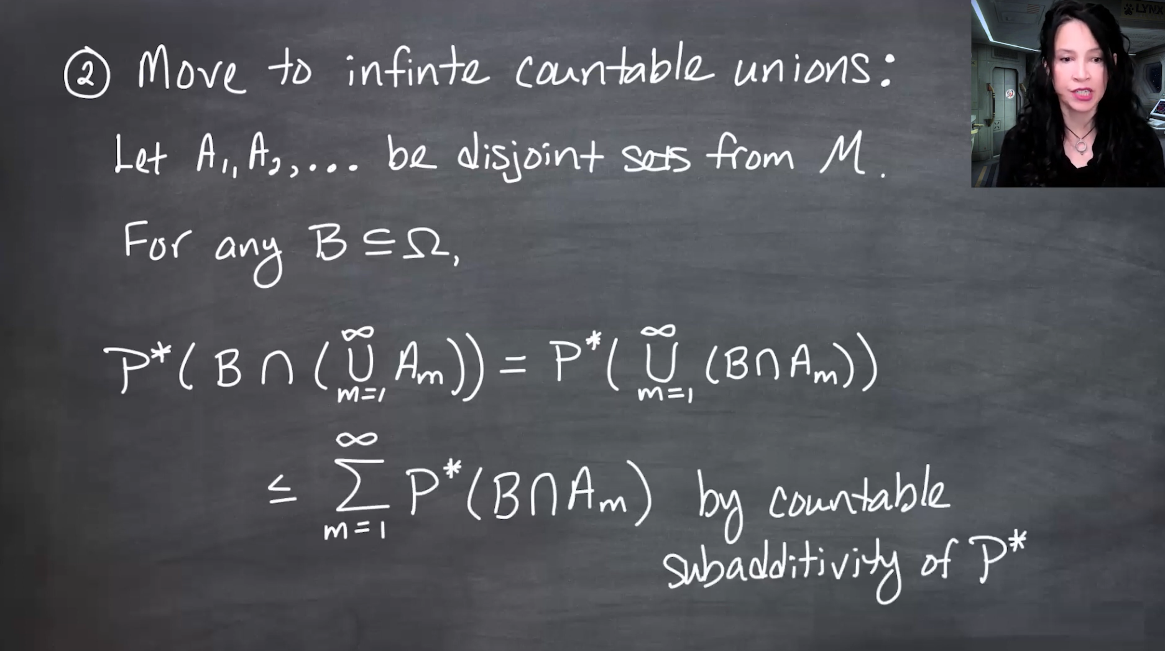
Now let A_1,A_2,\ldots\in\mathcal{M} be disjoint. We want

P^*\left(B\cap\bigcup_{n=1}^{\infty}A_n\right) = \sum_{n=1}^{\infty}P^*(B\cap A_n).

The \leq direction follows from countable subadditivity of P^*:

P^*\left(\bigcup_{n=1}^{\infty}(B\cap A_n)\right) \leq \sum_{n=1}^{\infty}P^*(B\cap A_n).

The less-than direction follows from countable subadditivity.

Figure 151.22: This direction uses only the general subadditivity property of P^*, which was proved before the lemma roadmap.

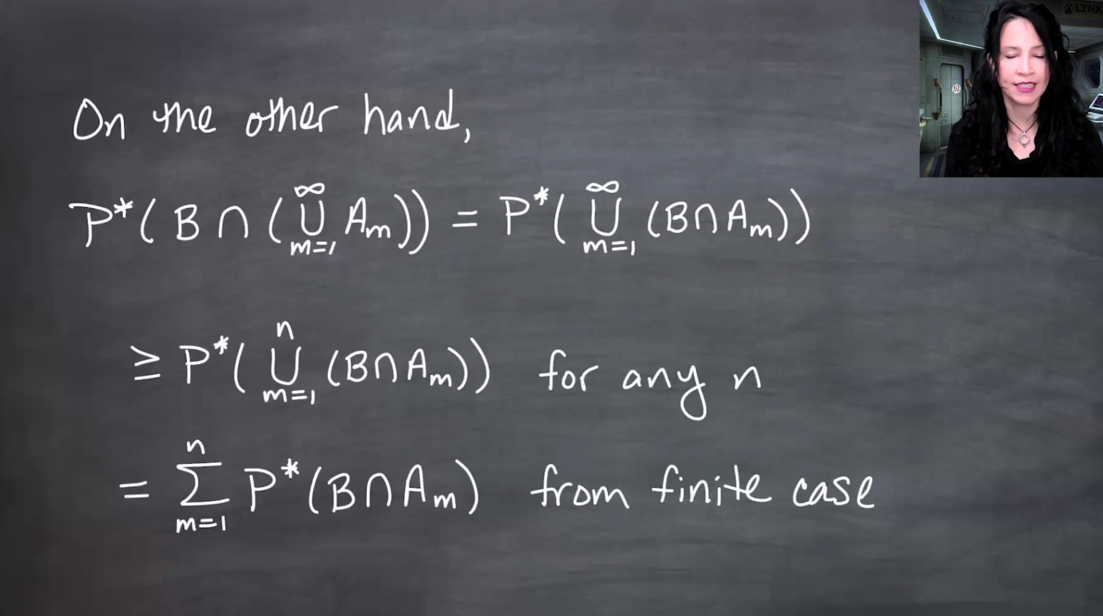
For the \geq direction, use monotonicity. For every finite m,

\bigcup_{n=1}^{m}(B\cap A_n) \subseteq \bigcup_{n=1}^{\infty}(B\cap A_n).

Therefore,

P^*\left(B\cap\bigcup_{n=1}^{\infty}A_n\right) \geq P^*\left(B\cap\bigcup_{n=1}^{m}A_n\right).

By the finite case,

P^*\left(B\cap\bigcup_{n=1}^{m}A_n\right) = \sum_{n=1}^{m}P^*(B\cap A_n).

The greater-than direction uses finite partial unions.

Figure 151.23: Every finite partial union is contained in the countable union. Monotonicity gives the inequality, and the finite case rewrites the right-hand side as a partial sum.

Letting m\to\infty gives

P^*\left(B\cap\bigcup_{n=1}^{\infty}A_n\right) \geq \sum_{n=1}^{\infty}P^*(B\cap A_n).

Together with the \leq direction, this proves equality.

Taking the limit of partial sums completes countable additivity.

Figure 151.24: The infinite sum is defined as the limit of its finite partial sums. This upgrades finite additivity on \mathcal{M} to countable additivity on disjoint sequences in \mathcal{M}.

Taking B=\Omega gives Lemma 2 exactly.

151.7 Lemma 3: \mathcal{M} is a sigma-field

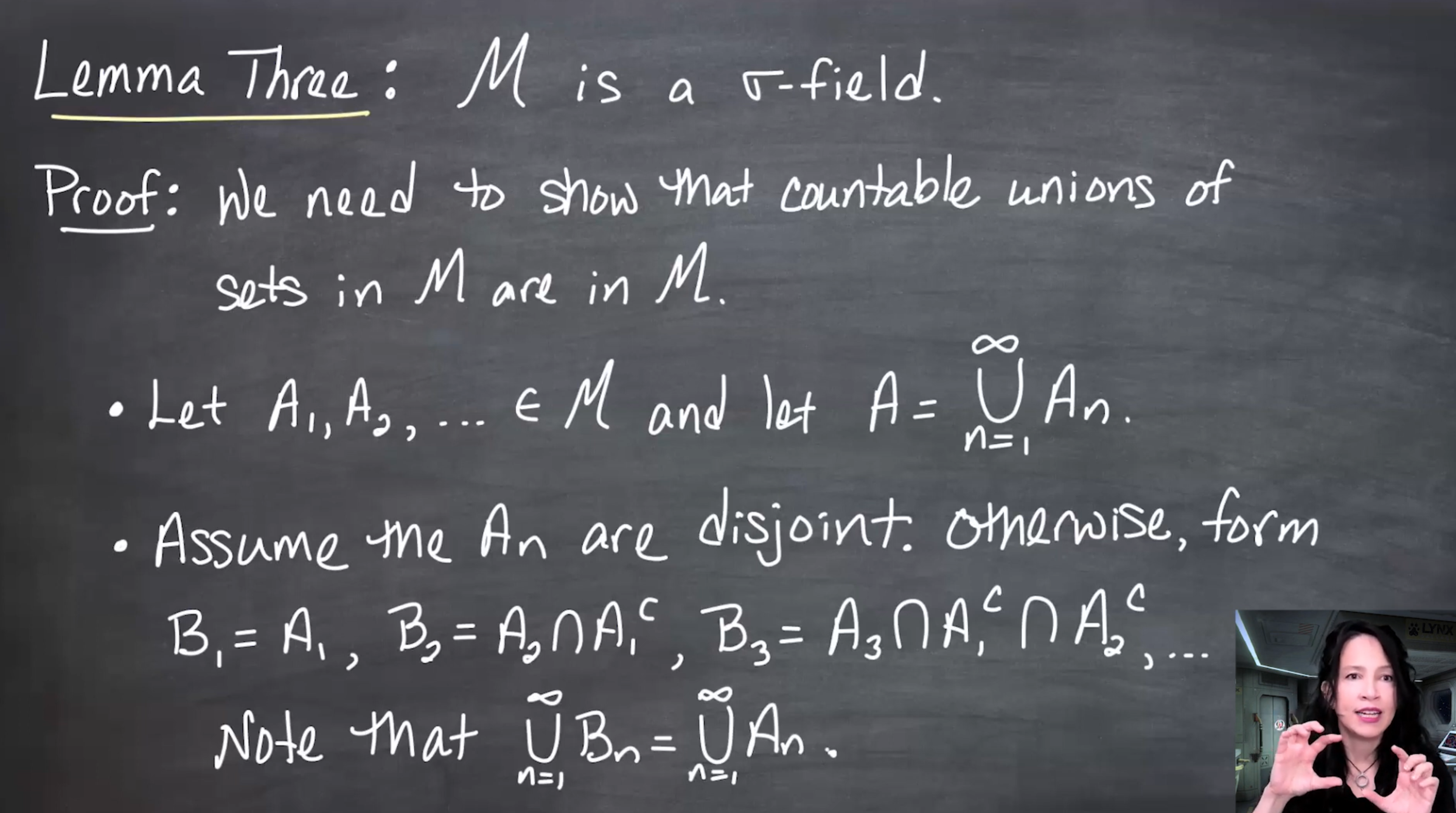
Lemma 151.3 (Lemma 3) The collection \mathcal{M} is a \sigma-field.

Lemma 1 already shows that \mathcal{M} is a field. Therefore, the only missing property is closure under countable unions.

Let

A=\bigcup_{n=1}^{\infty}A_n, \qquad A_n\in\mathcal{M}.

We must show A\in\mathcal{M}.

Lemma 3 reduces to countable union closure.

Figure 151.25: A field already has \Omega, complements, and finite unions. A \sigma-field additionally requires closure under countable unions.

The A_n need not be disjoint. But we can replace them by disjoint pieces:

B_1=A_1,

B_2=A_2\setminus A_1,

B_3=A_3\setminus(A_1\cup A_2),

and so on. These B_n are disjoint and have the same union as the original A_n.

Disjointizing a countable union.

Figure 151.26: The disjointization trick keeps the same total union while making Lemma 2 applicable.

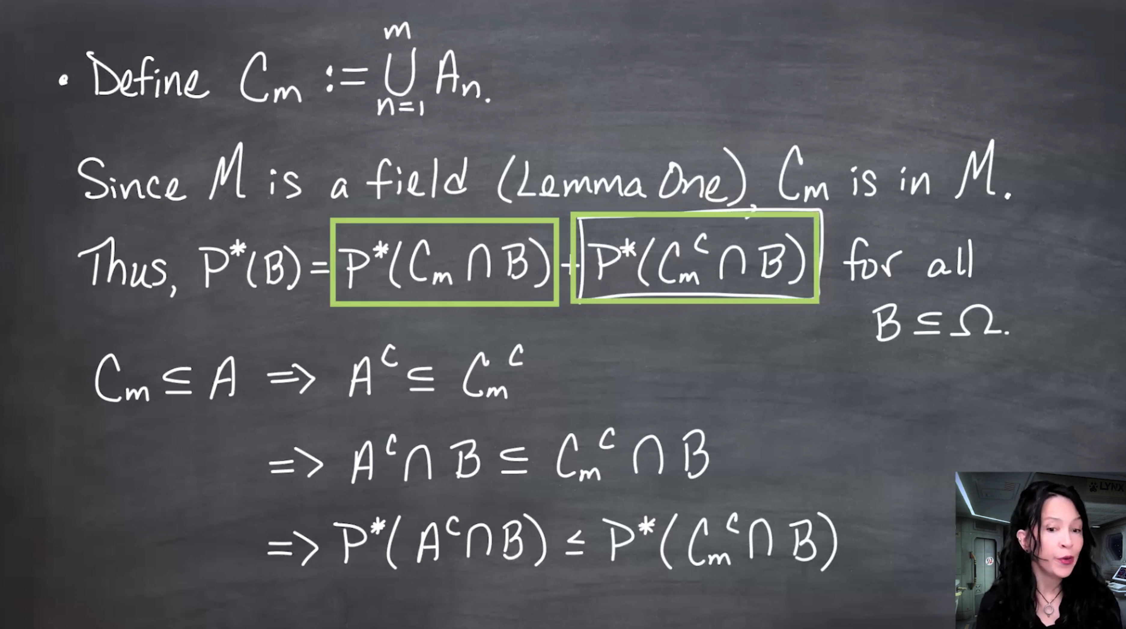
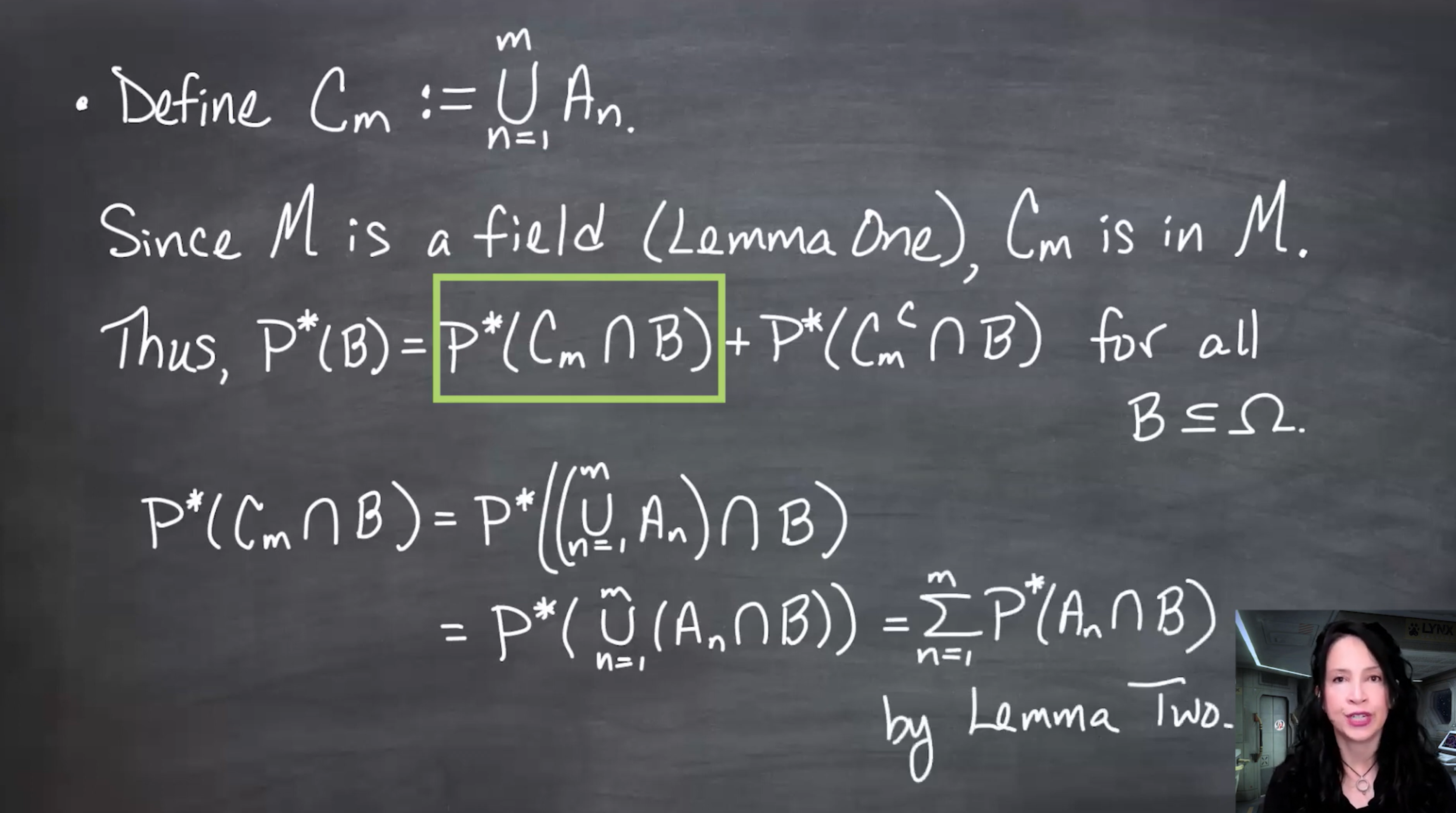
So assume the A_n are disjoint. Define the finite partial union

C_m=\bigcup_{n=1}^{m}A_n.

Since \mathcal{M} is a field, C_m\in\mathcal{M}.

For any B\subseteq\Omega, because C_m\in\mathcal{M},

P^*(B) = P^*(C_m\cap B)+P^*(C_m^c\cap B).

Now

C_m\cap B = \bigcup_{n=1}^{m}(A_n\cap B),

and by Lemma 2,

P^*(C_m\cap B) = \sum_{n=1}^{m}P^*(A_n\cap B).

Also, since C_m\subseteq A, we have A^c\subseteq C_m^c, hence

A^c\cap B\subseteq C_m^c\cap B.

By monotonicity,

P^*(A^c\cap B)\leq P^*(C_m^c\cap B).

Using finite partial unions C m to prove the full union is in M.

Figure 151.27: The proof compares the full countable union A with finite partial unions C_m. Lemma 2 handles the finite additive part, and monotonicity handles the complement term.

Putting these together,

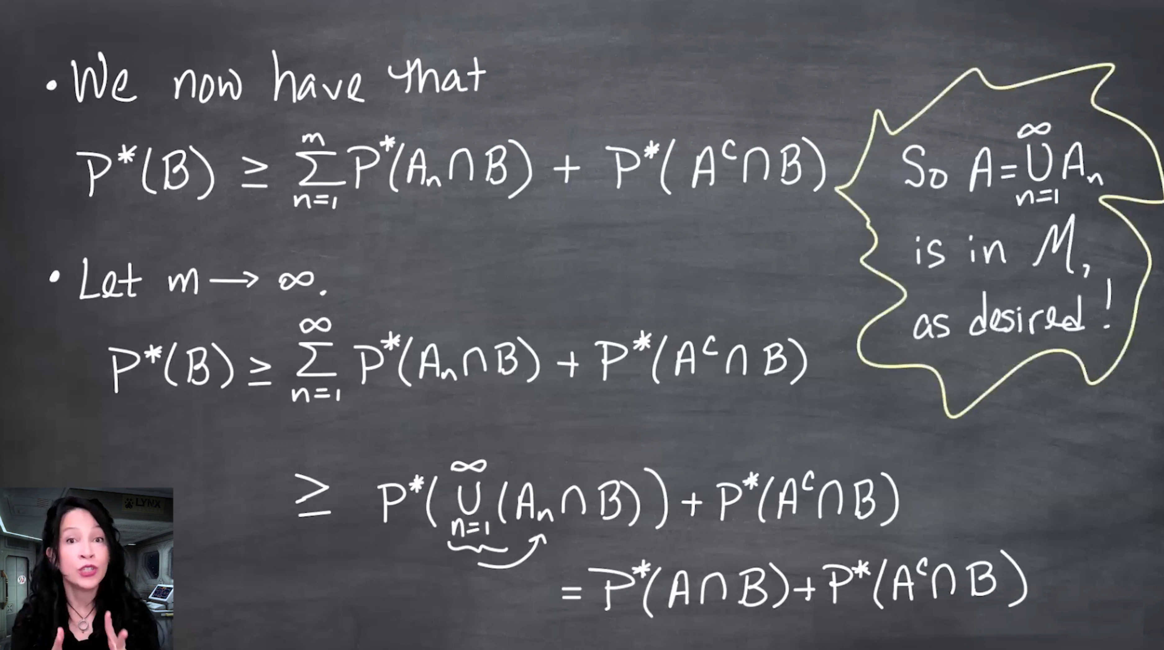
P^*(B) \geq \sum_{n=1}^{m}P^*(A_n\cap B)+P^*(A^c\cap B).

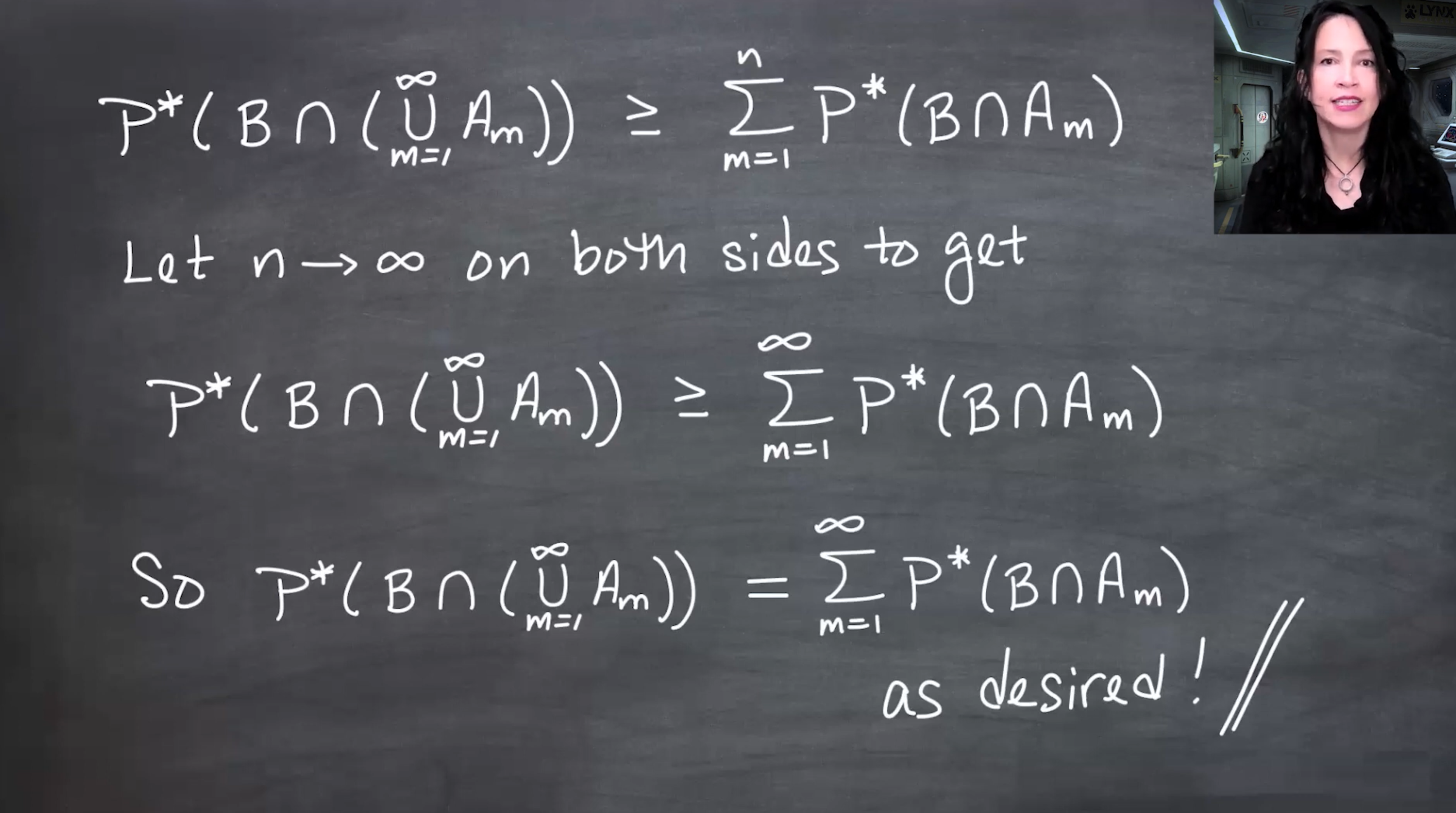
Letting m\to\infty,

P^*(B) \geq \sum_{n=1}^{\infty}P^*(A_n\cap B)+P^*(A^c\cap B).

By countable subadditivity,

\sum_{n=1}^{\infty}P^*(A_n\cap B) \geq P^*\left(\bigcup_{n=1}^{\infty}(A_n\cap B)\right) = P^*(A\cap B).

Therefore,

P^*(B) \geq P^*(A\cap B)+P^*(A^c\cap B).

This is the one-sided criterion for A\in\mathcal{M}. Hence \mathcal{M} is closed under countable unions.

Together with Lemma 1, this proves that \mathcal{M} is a \sigma-field.

151.8 Takeaway

This lesson proves the structural part of the extension theorem:

\mathcal{M} \text{ is a field} \quad\Longrightarrow\quad P^* \text{ is countably additive on } \mathcal{M} \quad\Longrightarrow\quad \mathcal{M} \text{ is a } \sigma\text{-field}.

The key proof pattern is:

1. define \mathcal{M} by a splitting identity;
2. use subadditivity of P^* to get one inequality for free;
3. prove the reverse inequality where needed;
4. use finite approximations and limits to move from finite to countable unions.

The next lesson proves Lemmas 4–6, which connect \mathcal{M} back to the original field \mathcal{F}_0 and complete the extension argument.