135 Lesson 1.3.4: Simulating correlated Gaussian random vectors

135.1 Generating correlated random vectors

• Straightforward to implement KF steps in Octave.
• To validate KF code via simulation, however, we also must simulate system whose state is being estimated.
  • Produces system input/output data as input to the KF.
  • Provides “true” state value at every point in time.
• But, to simulate the true system, must be able to create nonzero mean Gaussian noise with covariance \Sigma_{\tilde{Y}}.
• That is, we want \tilde{Y} \sim N(\bar{y}, \Sigma_{\tilde{Y}}) but randn.m returns X \sim N(0, I).
  • How to convert X to \tilde{Y}?

135.2 Functions of a random variable

Suppose we are given two random variables Y and X with Y = g(X).

Also assume that g^{-1} exists, and that g and g^{-1} are continuously differentiable. Then: f_Y(y) = f_X\!\left(g^{-1}(y)\right) \left|\det\!\left(\frac{\partial g^{-1}(y)}{\partial y}\right)\right|

where |\det(\cdot)| means to take the absolute value of the determinant.

So what? Suppose that X is a Gaussian random vector and we form some affine function of X such as: Y = AX + b.

• We can now form the PDF of Y → handy!
• This is going to be a key step in learning how to simulate correlated Gaussian random variables.

135.3 Example 1 with Gaussian

Let’s find the PDF of Y = AX + b in a couple of steps.

Start with scalar X and Y = kX, and X \sim N(0, \sigma_X^2).

Then X = \frac{1}{k}Y and so g^{-1}(y) = \frac{1}{k}y.

Also, \frac{\partial g^{-1}(y)}{\partial y} = \frac{1}{k}.

Therefore, f_Y(y) = f_X\!\left(\frac{y}{k}\right)\left|\frac{1}{k}\right| = \frac{1}{|k|}\frac{1}{\sqrt{2\pi}\sigma_X} \exp\!\left(-\frac{(y/k)^2}{2\sigma_X^2}\right) = \frac{1}{\sqrt{2\pi(\sigma_X k)^2}} \exp\!\left(-\frac{y^2}{2(\sigma_X k)^2}\right).

Therefore, multiplication by gain k results in a normally distributed random variable with scale change in standard deviation: Y \sim N(0, k^2\sigma_X^2).

135.4 Example 2 with Gaussian

Now, consider Y = AX + B where A is a constant (non-singular) matrix, B is a constant vector, and X \sim N(\bar{x}, \Sigma_{\tilde{X}}).

Then X = A^{-1}Y - A^{-1}B so g^{-1}(y) = A^{-1}y - A^{-1}B.

Also, \frac{\partial g^{-1}(y)}{\partial y} = A^{-1}.

The pdf of X is f_X(x) = \frac{1}{(2\pi)^{n/2}|\Sigma_{\tilde{X}}|^{1/2}} \exp\!\left[ -\frac{1}{2}(x-\bar{x})^T \Sigma_{\tilde{X}}^{-1}(x-\bar{x}) \right].

Therefore, f_Y(y) = |A^{-1}| \frac{1}{(2\pi)^{n/2}|\Sigma_{\tilde{X}}|^{1/2}} \exp\!\left[ -\frac{1}{2} \left(A^{-1}(y-B)-\bar{x}\right)^T \Sigma_{\tilde{X}}^{-1} \left(A^{-1}(y-B)-\bar{x}\right) \right].

We are going to simplify this expression on the next slide.

To do so, note that we can use standard properties of expectation to show that \bar{y} = A\bar{x} + B and \Sigma_{\tilde{Y}} = A\Sigma_{\tilde{X}}A^T.

135.5 Example 2 with Gaussian (cont)

Goal: simplify the following expression, knowing that \bar{y} = A\bar{x} + B \qquad\text{and}\qquad \Sigma_{\tilde{Y}} = A\Sigma_{\tilde{X}}A^T.

f_Y(y) = |A^{-1}| \frac{1}{(2\pi)^{n/2}|\Sigma_{\tilde{X}}|^{1/2}} \exp\!\left[ -\frac{1}{2} \left(A^{-1}(y-B)-\bar{x}\right)^T \Sigma_{\tilde{X}}^{-1} \left(A^{-1}(y-B)-\bar{x}\right) \right]

= \frac{1}{(2\pi)^{n/2}\left(|A||\Sigma_{\tilde{X}}||A^T|\right)^{1/2}} \exp\!\left[ -\frac{1}{2}(y-\bar{y})^T (A^{-1})^T \Sigma_{\tilde{X}}^{-1} A^{-1} (y-\bar{y}) \right]

= \frac{1}{(2\pi)^{n/2}|\Sigma_{\tilde{Y}}|^{1/2}} \exp\!\left[ -\frac{1}{2}(y-\bar{y})^T \Sigma_{\tilde{Y}}^{-1} (y-\bar{y}) \right].

Conclusion: Sum of Gaussians is Gaussian — very special case.

135.6 Application to our problem

Suppose that we can find matrix A such that A^T A = \Sigma_{\tilde{Y}}.

Then, we generate samples x of random vector X \sim N(0, I) and compute samples y of random vector Y = \bar{y} + A^T X.

Since X is zero-mean, E[Y] = E[\bar{y} + A^T X] = \bar{y}, as desired.

The covariance of Y is: E[(Y-\bar{y})(Y-\bar{y})^T] = E[(A^T X)(A^T X)^T]

= E[(A^T X)(X^T A)]

= A^T E[XX^T] A

= A^T I A = \Sigma_{\tilde{Y}}, also as desired.

135.7 Important matrix factorizations

So, if we can find A such that A^T A = \Sigma_{\tilde{Y}}, we can generate samples x of X \sim N(0, I) and compute y = \bar{y} + A^T x.

Three ways to generate A:

• Cholesky factorization of \Sigma_{\tilde{Y}} computes A such that A^T A = \Sigma_{\tilde{Y}} as long as \Sigma_{\tilde{Y}} is positive definite (all eigenvalues are strictly greater than zero).
• LDL factorization of \Sigma_{\tilde{Y}} produces L, D such that LDL^T = \Sigma_{\tilde{Y}} and requires only that \Sigma_{\tilde{Y}} be positive semi-definite. Can then compute A = \sqrt{D}\,L^T.
• LU factorization of \Sigma_{\tilde{Y}} produces L, U such that LU = \Sigma_{\tilde{Y}} and requires only that \Sigma_{\tilde{Y}} be positive semi-definite. Can then compute A = \operatorname{diag}\!\left(\sqrt{\operatorname{diag}(U)}\right)L^T.

Cholesky and LU are built into Octave; all are built into MATLAB.

135.8 Example Octave code

Suppose we wish to generate a single sample of y using the Cholesky method:

ybar = [1; 2];
covar = [1, 0.5; 0.5, 1];
A = chol(covar);
x = randn([2, 1]);
y = ybar + A' * x;

Suppose we wish to generate 5000 samples of y using the LU method:

ybar = [1; 2];
covar = [1, 0.5; 0.5, 1];
[L, U] = lu(covar);
A = diag(sqrt(diag(U))) * L';
x = randn([2, 5000]);
y = ybar(:, ones([1 5000])) + A' * x;
plot(y(1,:), y(2,:), '.');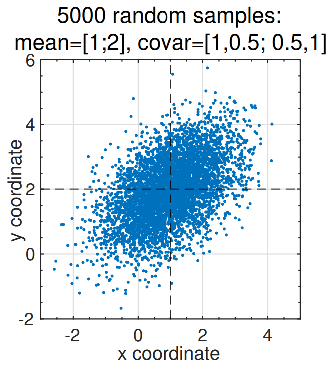

Figure 135.1: 5000 random samples scatter plot placeholder

135.9 Summary

• In order to test KF code via simulation, must also simulate system whose state is being estimated.
• This requires ability to simulate (possibly) correlated, (possibly nonzero mean) noises.
• Octave only natively produces samples of zero-mean uncorrelated Gaussians.
• But, it can efficiently transform these to have desired mean and correlation using a matrix determined using either the Cholesky or LU matrix decompositions, both of which are built into Octave.