130.1 Is it even possible for a KF to estimate this model’s state?
130.1.1 Observability: Can I estimate an initial state?
- We define a system to be observable if we can determine its initial state vector x(0) via processing its input signal u(t) and its output signal z(t).
- Since we can simulate the system’s state and output if we know x(0) and u(t), this also implies that we can determine x(t) for all t \geq 0.
x(t) = e^{At} x(0) + \int_0^t e^{A(t-\tau)} B u(\tau) d\tau - So, it should not be surprising that a system must be observable for the KF to work (noting an exception to this rule that is stated on the summary slide). - How do we determine whether a system is observable?
130.1.2 Finding an equation describing output derivatives
Consider a brute-force approach. Suppose we have the model:
\begin{aligned} \dot x(t) &= A x(t) + B u(t) \\ z(t) &= C x(t) + D u(t) \end{aligned}
and we have initial conditions z(0), \dot{z}(0), \ddot{z}(0), u(0), \dot{u}(0), and \ddot{u}(0).
- How can we determine x(0) from these initial conditions? \begin{aligned} z(0) &= C x(0) + D u(0), \\ \dot{z}(0) &= C (\underbrace{A x(0) + B u(0)}_{\dot{x}(0)}) + D \dot{u}(0) = C A x(0) + C B u(0) + D \dot{u}(0), \\ \ddot{z}(0) &= C A^2 x(0) + C A B u(0) + C B \dot{u}(0) + D \ddot{u}(0) \end{aligned}
In general (where superscript parentheses indicate derivatives, not powers), z^{(k)}(0) = C A^k x(0) + C A^{k-1} B u(0) + \dots + C B u^{k-1}(0) + D u^{(k)}(0),
130.1.3 The Observability matrix \mathcal{O}
- We can write this compactly in matrix form (for n D 3): \begin{bmatrix}z(0) \\ \dot{z}(0) \\ \ddot{z}(0) \end{bmatrix} = \underbrace{\begin{bmatrix} C \\ CA \\ CA^2 \end{bmatrix}}_{\mathcal{O}(C,A)} x(0) + \underbrace{\begin{bmatrix} D & 0 & 0 \\ CB & D & 0 \\ CAB & CB & D \end{bmatrix}}_{\mathcal{T}(C,A,B,D)} \begin{bmatrix} u(0) \\ \dot{u}(0) \\ \ddot{u}(0) \end{bmatrix} where \mathcal{T} is a (block) “Toeplitz matrix” (in general, \mathcal{O} has n (block) rows).
- Thus, if the observability matrix \mathcal{O} is invertible, then: x(0) = \mathcal{O}^{-1} \left( \begin{bmatrix}z(0) \\ \dot{z}(0) \\ \ddot{z}(0) \end{bmatrix} - \mathcal{T} \begin{bmatrix} u(0) \\ \dot{u}(0) \\ \ddot{u}(0) \end{bmatrix} \right)
- We say that \{C,A\} is an observable pair if \mathcal{O} is nonsingular (for multi-input multi-output systems, \mathcal{O} must be full rank).
130.1.4 A brute-force continuous-time observer
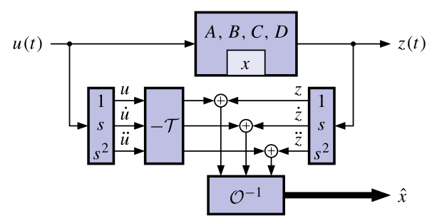
- One possible approach to determine the system state, directly from the equations, uses differentiators.
- A big problem is that differentiators amplify noise, corrupting the state estimate.
- The KF is a more practical observer that doesn’t use differentiators.
- Regardless of the approach, it turns out that the system must be observable to be able to determine its initial state.
- CONCLUSION: If \mathcal{O} is nonsingular, we can determine/estimate the initial state x(0) of the system using only u(t) and z(t) (and so we can estimate x(t) for all t \geq 0).
- ADVANCED TOPIC: If some states are unobservable but stable, an observer will still converge to the true state, although x(0) may not be uniquely determined.
130.1.5 Examples of unobservable models
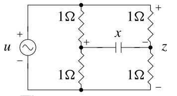
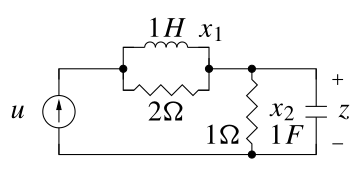
Consider the following two unobservable circuits:
The state-space model for the first circuit is:
\begin{aligned} \dot{x}(t) &= - \frac{1}{C} x(t) + \frac{1}{C} u(t) \\ z(t) &= u(t) \end{aligned}
- Notice that z(t) is not a function of x(t). The state-space model output equation has C matrix equal to zero. Therefore, \mathcal{O} = 0. Not observable.
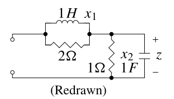
- In the second circuit, if u(t) = 0, x_1(0) \neq 0 and x_2(0) = 0, then \dot{z}(t) = 0 and we cannot determine x_1(0) (circuit redrawn for u(t) = 0).
130.1.6 Controllability: Can I get there from here?
Controllability is a dual idea to observability. We won’t go into depth here since it is not as important for our topic of study.
Controllability asks the question, “Can I move from any initial state to any desired state via suitable selection of the control input u.t/?”
The answer boils down to a condition on a matrix called the controllability matrix C = [B\; AB\; \cdots\; A^{N-1}B]
TEST: If C is nonsingular, then the system is controllable.
130.2 Diagonal systems, controllability and observability
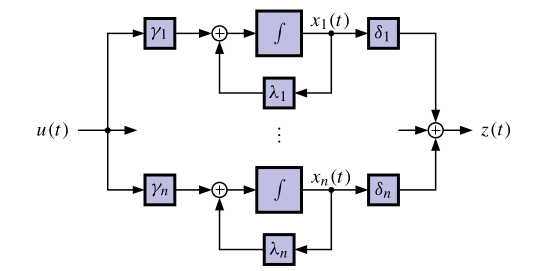
We can gain insight by considering a system in diagonal form:
\begin{aligned} \dot{x}(t) &= \begin{bmatrix} \lambda_1 & 0 & \cdots & 0 \\ 0 & \lambda_2 & \cdots & 0 \\ \vdots & \vdots & \ddots & \vdots \\ 0 & 0 & \cdots & \lambda_n \end{bmatrix} x(t) + \begin{bmatrix} \gamma_1 \\ \gamma_2 \\ \vdots \\ \gamma_n \end{bmatrix} u(t) \\ z(t) &= \begin{bmatrix} \delta_1 & \delta_2 & \cdots & \delta_n \end{bmatrix} x(t) + d u(t) \end{aligned}
- When controllable? When observable?
\mathcal{O} = \begin{bmatrix} C \\ CA \\ \vdots \\ CA^{n-1} \end{bmatrix} =\begin{bmatrix} \delta_1 & \delta_2 & \cdots & \delta_n \\ \lambda_1 \delta_1 & \lambda_2 \delta_2 & \cdots & \lambda_n \delta_n \\ \vdots & \vdots & \ddots & \vdots \\ \lambda_1^{n-1} \delta_1 & \lambda_2^{n-1} \delta_2 & \cdots & \lambda_n^{n-1} \delta_n \end{bmatrix} \\ = \underbrace{\begin{bmatrix} 1 & 1 & \cdots & 1 \\ \lambda_1 & \lambda_2 & \cdots & \lambda_n \\ \vdots & \vdots & \ddots & \vdots \\ \lambda_1^{n-1} & \lambda_2^{n-1} & \cdots & \lambda_n^{n-1} \end{bmatrix}}_{\text{Vandermonde matrix } \mathcal{V}} \begin{bmatrix} \delta_1 & 0 & \cdots & 0 \\ 0 & \delta_2 & \cdots & 0 \\ \vdots & \vdots & \ddots & \vdots \\ 0 & 0 & \cdots & \delta_n \end{bmatrix}
130.2.1 Why is a system unobservable? Uncontrollable?
- Is the observability matrix singular?
\det\{\mathcal{O}\} = ( \delta_1 \cdots \delta_n ) \det\{\mathcal{V}\} = ( \delta_1 \cdots \delta_n ) \prod_{1 \leq i < j \leq n} (\lambda_j - \lambda_i)
- Observable \iff \lambda_i \neq \lambda_j \forall i \neq j and \delta_i \neq 0 \forall i.
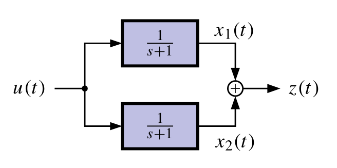
- If \lambda_1 = \lambda_2 then not observable. Can only “observe” the sum x_1 + x_2.
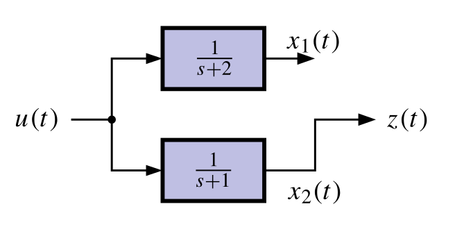
- If \delta_k = 0 then not observable. Cannot observe mode k.
- What about controllability? Analysis is similar: just switch the roles of the \gammas and \lambdas.
- Controllable \iff \lambda_i \neq \lambda_j \forall i \neq j and \gamma_i \neq 0 \forall i.
- If \gamma_1 = \gamma_2 then not controllable. Can only “control” the sum x_1 + x_2.
- If \gamma_k = 0 then cannot control mode k.
130.2.2 Equations describing discrete-time outputs
- Can we reconstruct x_0 from the output z_k and input u_k ?
\begin{align} z_{k} &= C x_{k} + D_d u_{k} \text {so}\\ z_{0} &= C[A x_{0} + B u_0]+ D u_{0} \\ z_{1} &= C[A^2 x_{0} + A B u_0 + B u_1]+ D u_{1} \\ \vdots \\ z_{n-1} &=C[A^{n-1} x_0 + A^{n-2} B u_0 + \cdots + B u_{n-2}]+ D u_{n-1} \end{align}
- In matrix/vector form, we can write: \begin{bmatrix} z_0 \\ z_1 \\ \vdots \\ z_{n-1} \end{bmatrix} = \underbrace{\begin{bmatrix} C \\ CA \\ \vdots \\ CA^{n-1} \end{bmatrix}}_{\mathcal{O}(C,A)} x_0 + \underbrace{\begin{bmatrix} D & 0 & \cdots & 0 \\ CB & D & \cdots & 0 \\ \vdots & \vdots & \ddots & \vdots \\ CA^{n-2}B & CA^{n-3}B & \cdots & D \end{bmatrix}}_{\mathcal{T}(C,A,B,D)} \begin{bmatrix} u_0 \\ u_1 \\ \vdots \\ u_{n-1} \end{bmatrix}
130.2.3 Discrete-time observability matrix
- So, similar to continuous-time, we write x_0 = \mathcal{O}^{-1} \left( \begin{bmatrix} z_0 \\ z_1 \\ \vdots \\ z_{n-1} \end{bmatrix} - \mathcal{T} \begin{bmatrix} u_0 \\ u_1 \\ \vdots \\ u_{n-1} \end{bmatrix} \right)
- If \mathcal{O} is invertible, x_0 may be found for any z_k ; u_k , and so the system is observable; also, we say that \{C, A\} forms an observable pair.
- Do more measurements of z_n; z_{n+1}; \dots help in reconstructing x_0?
- No! (Advanced topic: the Caley–Hamilton theorem).
- So, if the original state is not observable with n measurements, then it will not be observable with more than n measurements either.
- There is a structural problem where either a state is not connected (at all) to the output, or multiple states have the same eigenvalues (time constants).
130.2.4 A brute-force discrete-time observer
Since we know u_k and the dynamics of the system, if the system is observable we can determine the entire state sequence x_k , k \ge 0 once we determine x_0 \begin{aligned} x_n &= A^n x_0 + \sum_{i=0}^{n-1} A^{n-1-i} B u_i \\ &= A^n \mathcal{O}^{-1} \left( \begin{bmatrix} z_0 \\ z_1 \\ \vdots \\ z_{n-1} \end{bmatrix} - \mathcal{T} \begin{bmatrix} u_0 \\ u_1 \\ \vdots \\ u_{n-1} \end{bmatrix} \right) + \mathcal{C} \begin{bmatrix} u_0 \\ u_1 \\ \vdots \\ u_{n-1} \end{bmatrix} \end{aligned}
This is a perfectly good observer! (no differentiators…).
But it is still not nearly as good as the Kalman filters we will develop when there is noise present.
130.2.5 Discrete-time controllability
- On the previous slide, I condensed the convolution sum \sum_{i=0}^{n-1} A^{n-1-i} B u_i = \mathcal{C} \begin{bmatrix} u_{n-1} \\ \vdots \\ u_0 \end{bmatrix} using a discrete-time controllability matrix, which I now define explicitly
- The discrete-time controllability matrix is formed by (where we use the discrete-time A and B matrices):
\mathcal{C} = \begin{bmatrix} B & AB & \cdots & A^{n-1}B \end{bmatrix}
The matrix \mathcal{C} is invertible iff the system is controllable.
Similar concept for discrete-time compared to continuous-time (and again, we won’t make much use of it in this specialization).
130.2.6 Summary
- Is it even possible to estimate the state of our model?
- The (continuous- or discrete-time) observability matrix \mathcal{O} tells us whether the initial state can be found using measurements of input and output.
- If \mathcal{O} is invertible, the system is observable and we can find x(0) or x_0.
- If \mathcal{O} is not invertible, we cannot find x(0) or x_0 uniquely because either a state is not connected to the output or multiple states have the same eigenvalues.
- If we can find the initial state, we can compute it at any other time. Otherwise, we cannot compute the state uniquely at any other time.
- Therefore, we will say and assume that it is necessary for our models be observable for the KF to be able to estimate the state. 1
Advanced topic: A system is detectable if all states that cannot be observed are stable. We can apply KF to a detectable system (as the unobservable states decay toward a known trajectory in the absence of process noise) but uncertainties of unobservable states will generally become large.↩︎