150 L05 : Extending Probability Measures to Countable Additivity — Continued

Video 150.1: Lesson 5: the outer-measure roadmap for extending P from a field \mathcal{F}_0 to the generated \sigma-field \mathcal{F}=\sigma(\mathcal{F}_0).

150.1 Lesson map

• 0:12 — Recap: extend a probability measure from a field \mathcal{F}_0 to \sigma(\mathcal{F}_0).
• 1:08 — The outer-measure idea: cover arbitrary A\subseteq\Omega by sets from \mathcal{F}_0.
• 3:37 — Definition of the outer measure P^*.
• 5:17 — What extension means: preserve old values on \mathcal{F}_0.
• 6:09 — Recap of the four known properties of P^*.
• 9:13 — Motivation: splitting a set B by A and A^c.
• 10:17 — Define the collection \mathcal{M} of sets that split every B correctly.
• 11:15 — Equivalent definition of \mathcal{M} using only one inequality.
• 13:04 — Proof roadmap: six lemmas.
• 16:59 — How the lemmas imply the desired extension theorem.
• 20:29 — Uniqueness of the extension.
• 25:14 — Stronger uniqueness theorem and future \pi-systems.

150.2 Recap: the outer-measure construction

Covering an arbitrary set from outside.

Figure 150.1: The set A may not itself be in \mathcal{F}_0, so P(A) may not be defined. The workaround is to cover A using sets A_n\in\mathcal{F}_0 and use the known values P(A_n).

Disjoint covers may not be optimal.

Figure 150.2: Requiring covering sets to be disjoint is not necessarily better. A disjoint cover can include much more material outside A, so the construction considers all countable covers and lets the infimum choose the best upper estimate.

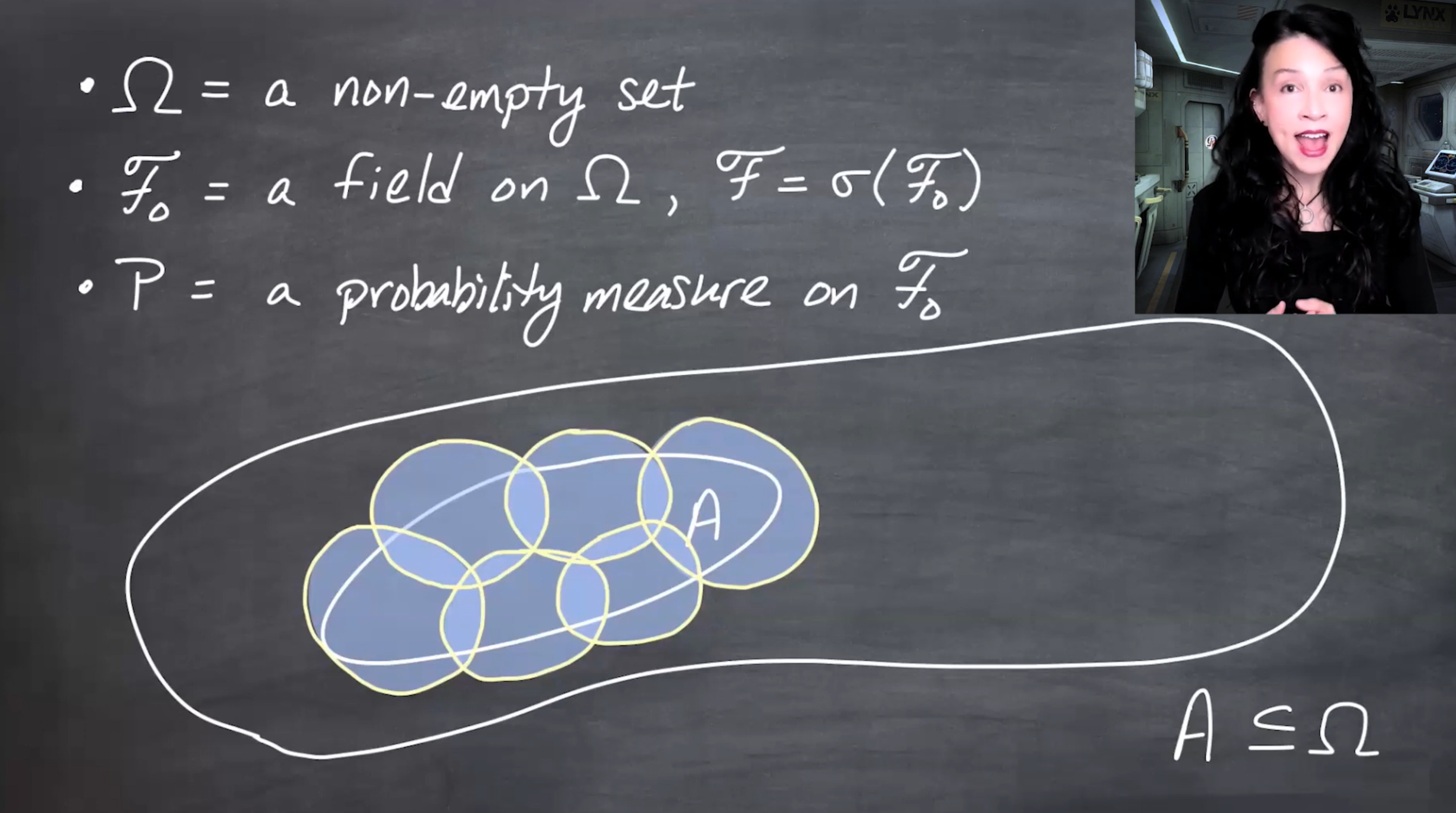
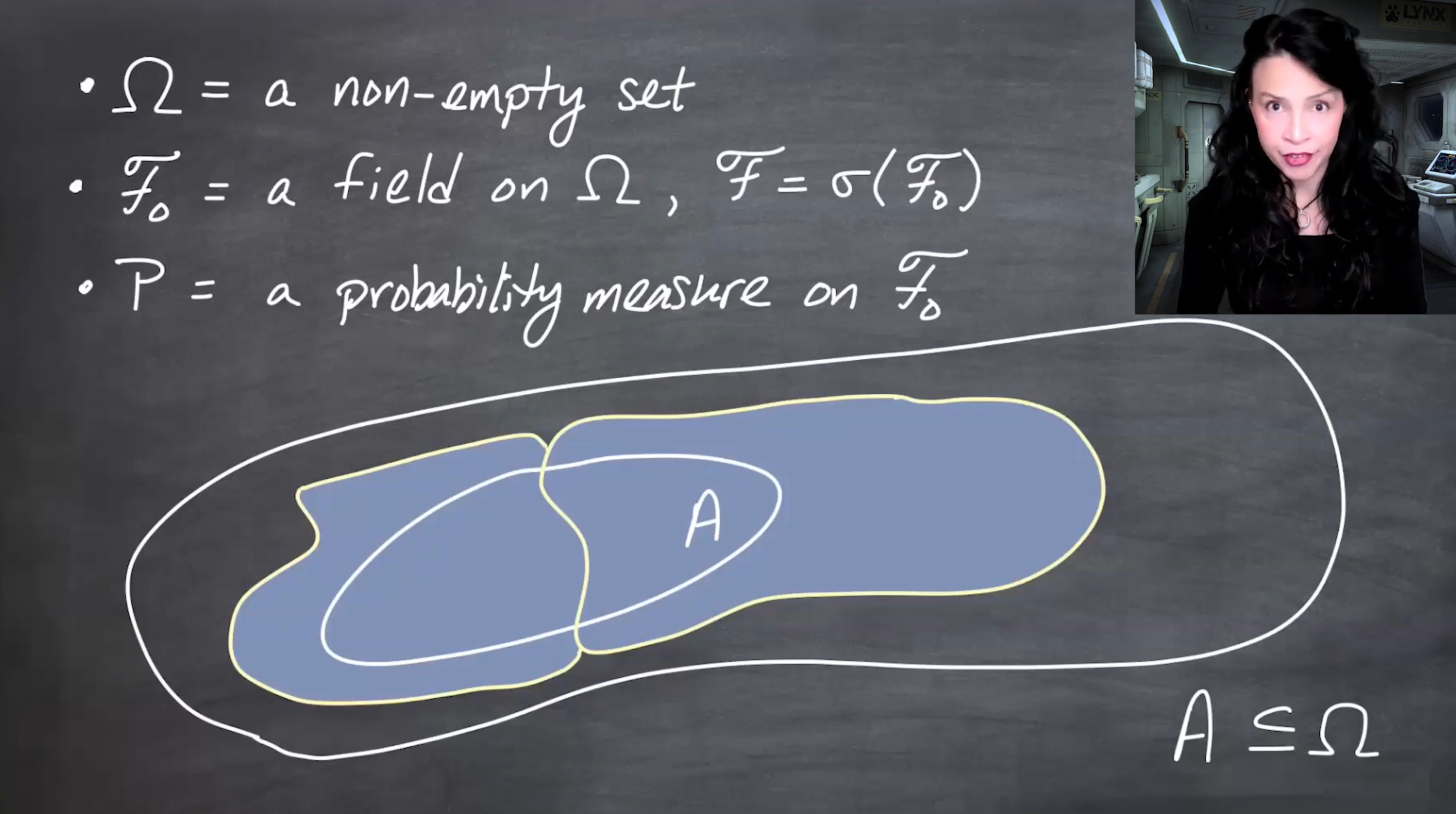
The previous lesson started with:

\Omega\neq\emptyset, \qquad \mathcal{F}_0 \text{ a field on } \Omega, \qquad \mathcal{F}=\sigma(\mathcal{F}_0),

and a probability measure

P:\mathcal{F}_0\to[0,1].

The goal is to extend P to the larger \sigma-field \mathcal{F}.

For an arbitrary subset A\subseteq\Omega, the idea was to cover A by countably many sets from \mathcal{F}_0, because those are the sets whose probabilities are already known.

The cover may include extra regions outside A, and the covering sets may overlap. So the sum of their probabilities is usually an overestimate.

150.3 Outer measure P^*

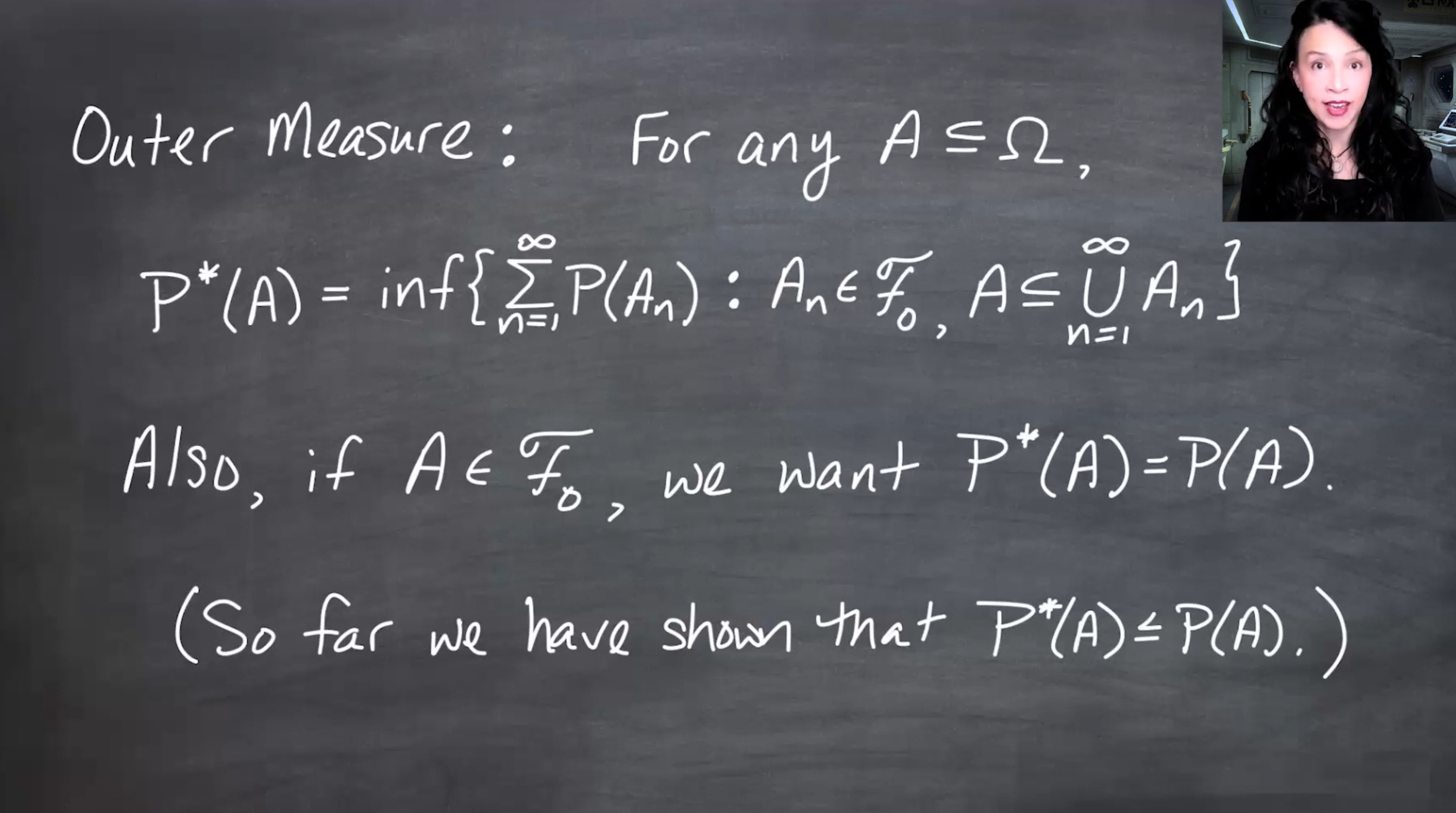
Definition 150.1 (Outer measure associated with P) For every subset A\subseteq\Omega, define

P^*(A) = \inf\left\{ \sum_{n=1}^{\infty}P(A_n) : A_n\in\mathcal{F}_0 \text{ and } A\subseteq\bigcup_{n=1}^{\infty}A_n \right\}.

This is called an outer measure because it approaches A from outside: cover A by measurable pieces from \mathcal{F}_0, sum their probabilities, and take the best possible upper bound.

Definition of the outer measure P star.

Figure 150.3: The formula for P^* is defined for every A\subseteq\Omega, even if A is not in \mathcal{F}_0 or in \mathcal{F}=\sigma(\mathcal{F}_0).

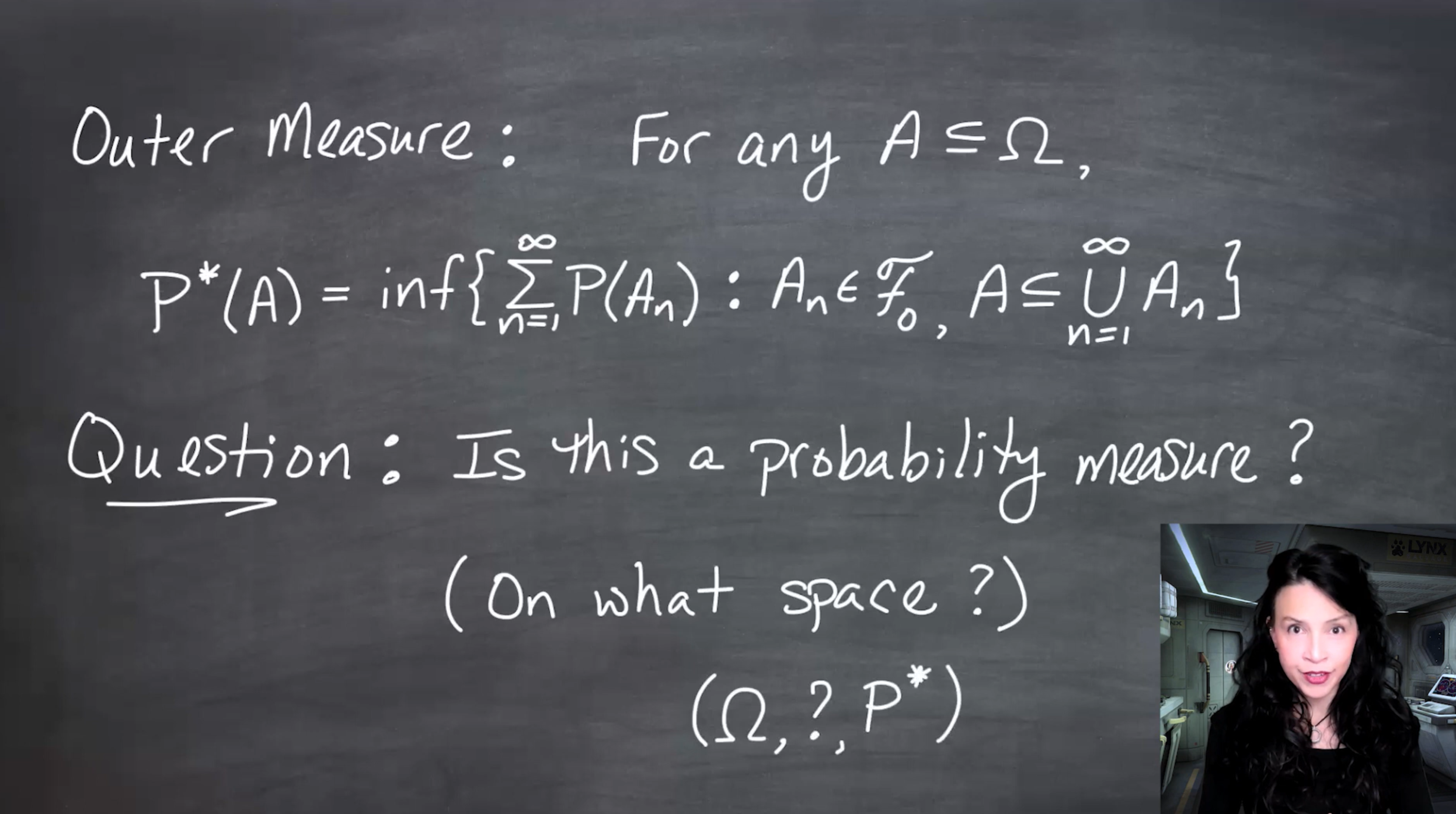
At this point, the terminology is slightly optimistic. We have called P^* an outer measure, but we have not yet proved that it behaves like a probability measure on the \sigma-field we care about.

150.4 What extension should mean

An extension must do two things:

1. assign values to more sets;
2. preserve the old values.

So for every A\in\mathcal{F}_0, we want

P^*(A)=P(A).

So far, the previous lesson only proved one direction:

P^*(A)\leq P(A) \qquad (A\in\mathcal{F}_0).

An extension must preserve the original probability values.

Figure 150.4: Calling P^* an extension means it should not disturb the probabilities already assigned by P on the field \mathcal{F}_0.

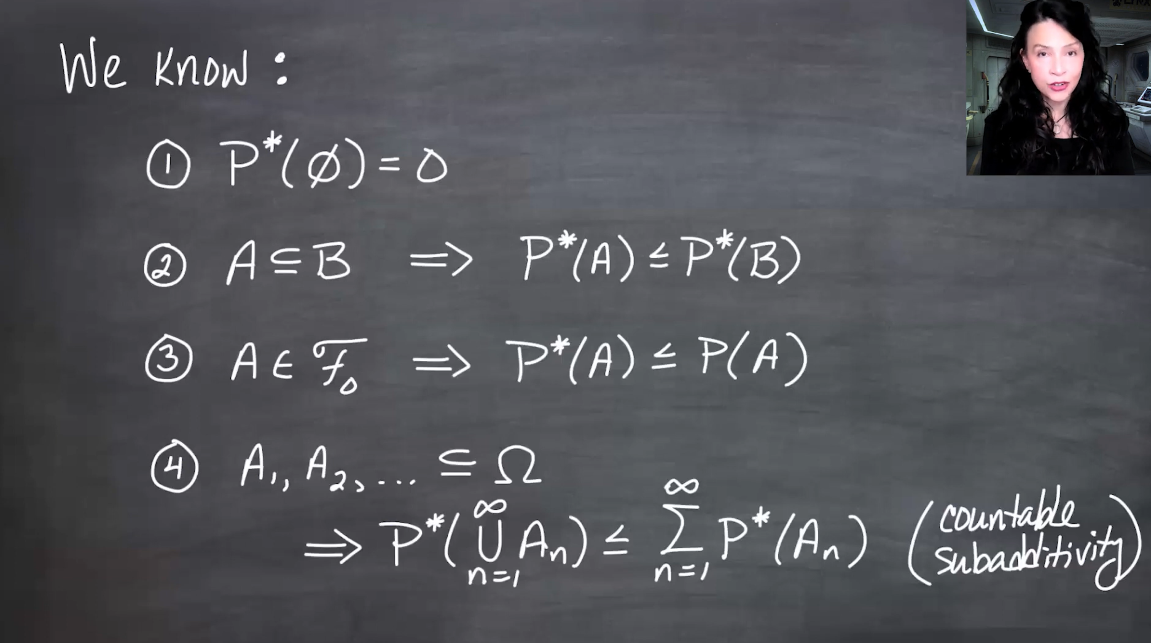
150.5 Four known properties of P^*

From Lesson 4, we know:

1. P^*(\emptyset)=0.
2. If A\subseteq B, then P^*(A)\leq P^*(B).
3. If A\in\mathcal{F}_0, then P^*(A)\leq P(A).
4. P^* is countably subadditive:

P^*\left(\bigcup_{n=1}^{\infty}A_n\right) \leq \sum_{n=1}^{\infty}P^*(A_n).

The first three known properties of P star.

Figure 150.5: These are measure-like properties, but they do not yet prove that P^* is a probability measure.

Countable subadditivity of P star.

Figure 150.6: Countable subadditivity is weaker than countable additivity. A probability measure needs equality for countable unions of disjoint measurable sets.

The missing pieces are:

• countable additivity on the right class of sets;
• P^*(\Omega)=1;
• equality P^*(A)=P(A) for A\in\mathcal{F}_0;
• identifying the \sigma-field on which P^* is a probability measure.

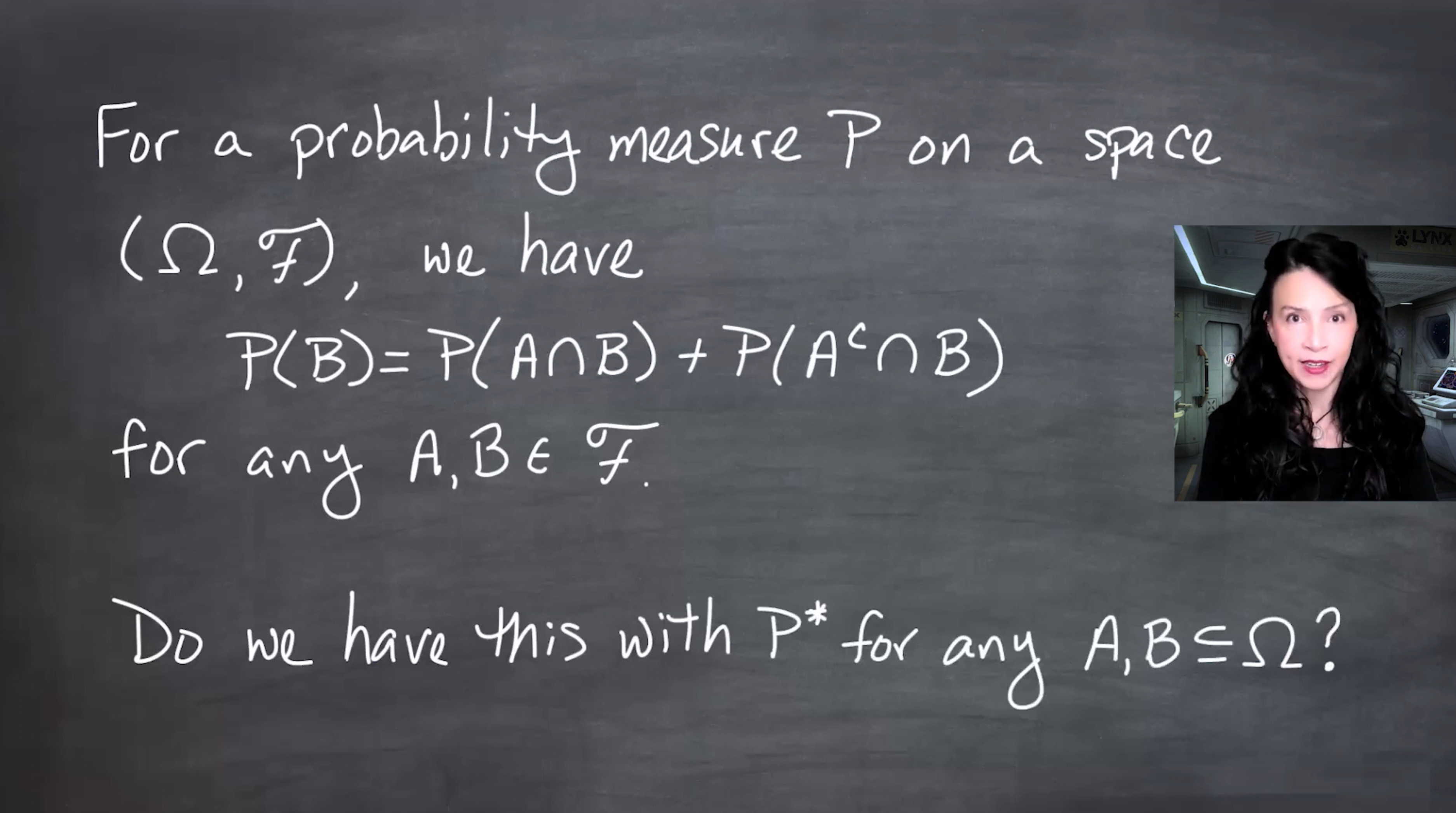
150.6 Splitting a set by A and A^c

For an actual probability measure, every measurable set B can be split into the part inside A and the part outside A:

B = (A\cap B)\cup(A^c\cap B),

where the two pieces are disjoint. Therefore,

P(B) = P(A\cap B)+P(A^c\cap B).

Splitting B into the part inside A and the part outside A.

Figure 150.7: For a genuine measure, cutting B by A should not create or destroy mass: the measure of B equals the sum of the measures of the two disjoint pieces.

This motivates defining the sets for which P^* has this splitting property.

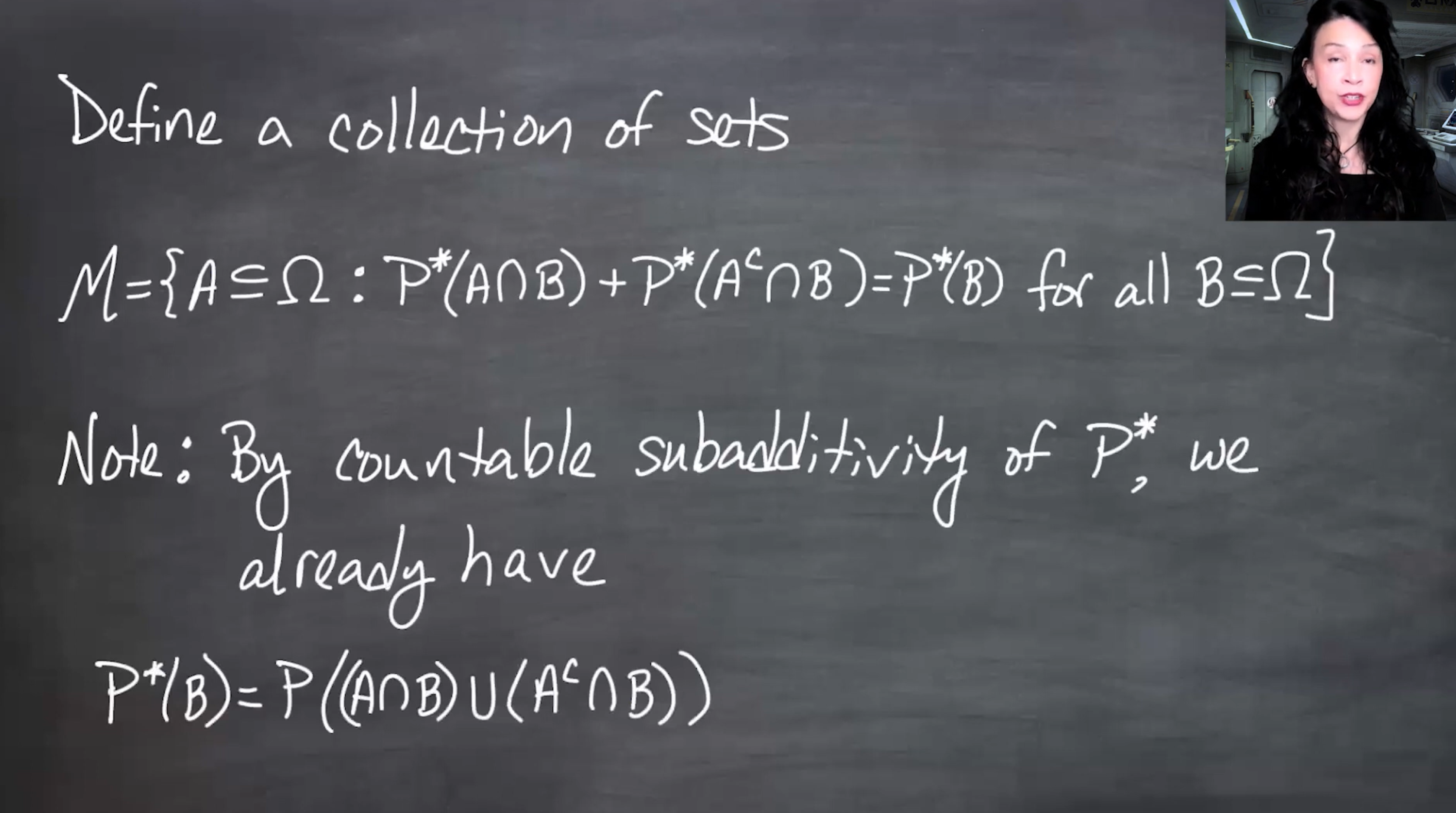
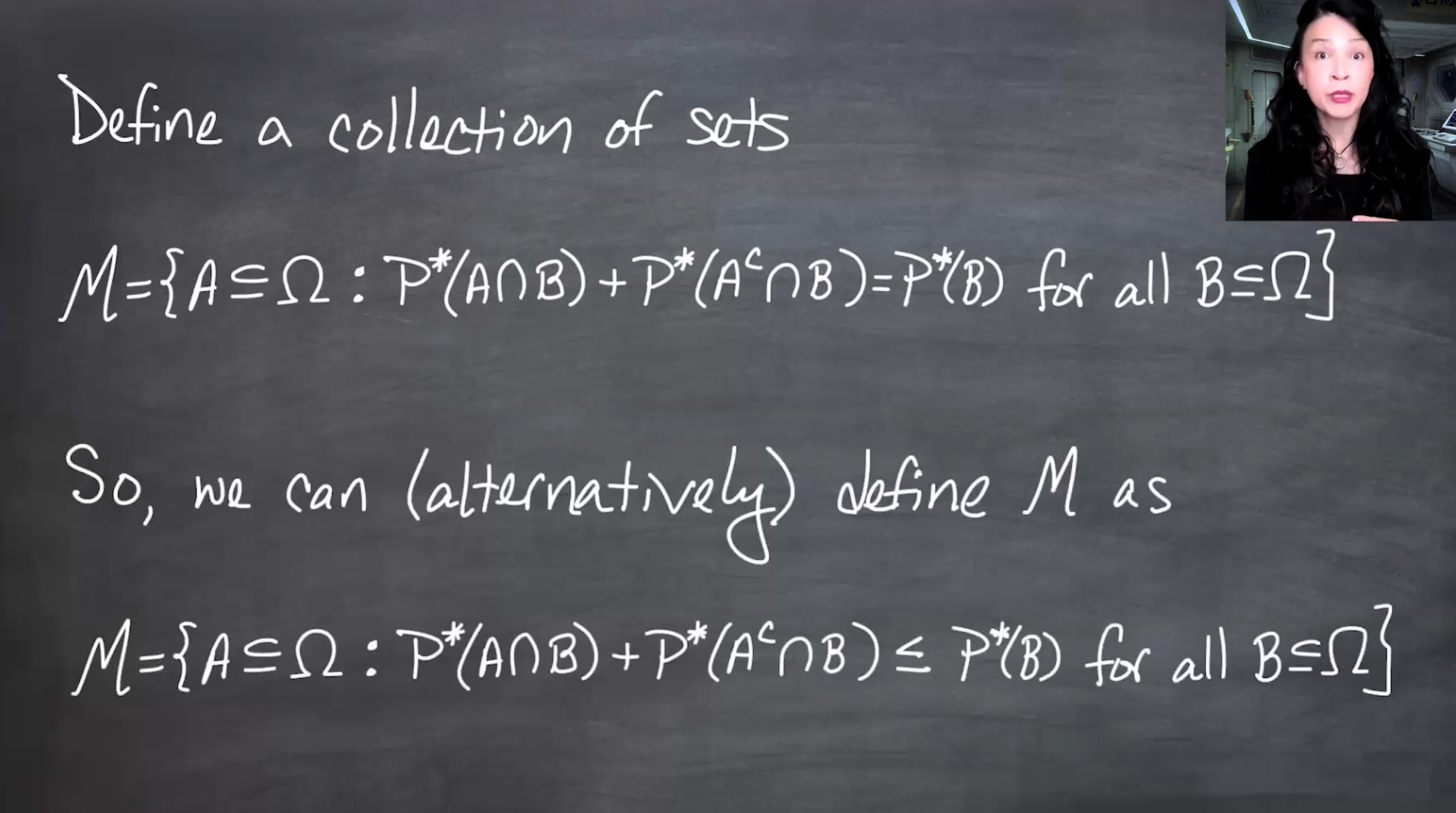
150.7 The collection \mathcal{M}

Definition 150.2 (The collection \mathcal{M}) Define \mathcal{M} to be the collection of all subsets A\subseteq\Omega such that, for every B\subseteq\Omega,

P^*(B) = P^*(A\cap B)+P^*(A^c\cap B).

These are the sets that split every test set B correctly under P^*.

Definition of the collection M.

Figure 150.8: The class \mathcal{M} collects the sets that are compatible with P^* in the sense that they divide every B into two additive pieces.

This is the Carathéodory-style measurability condition, although the lesson introduces it operationally rather than as a named theorem.

150.7.1 Equivalent one-sided condition

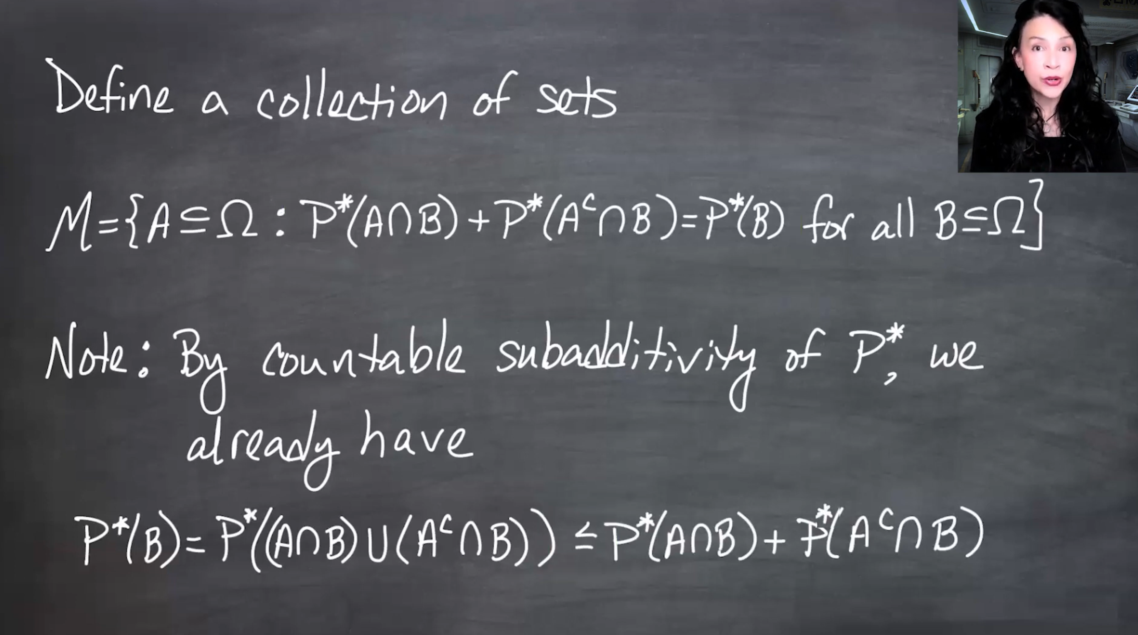
By countable subadditivity,

P^*(B) \leq P^*(A\cap B)+P^*(A^c\cap B)

always holds, because B=(A\cap B)\cup(A^c\cap B).

Therefore, to show equality it is enough to prove the reverse inequality:

P^*(A\cap B)+P^*(A^c\cap B) \leq P^*(B).

The reverse inequality is enough to define M.

Figure 150.9: The equality definition and the one-sided inequality definition of \mathcal{M} are equivalent because subadditivity already supplies the other inequality.

150.8 Roadmap: six lemmas

The proof that P^* extends P is long, so the lesson organizes it into six lemmas.

Lemma roadmap, first half.

Figure 150.10: The first three lemmas build the measurable world for P^*: show that \mathcal{M} is first a field, then closed under countable unions, hence a \sigma-field.

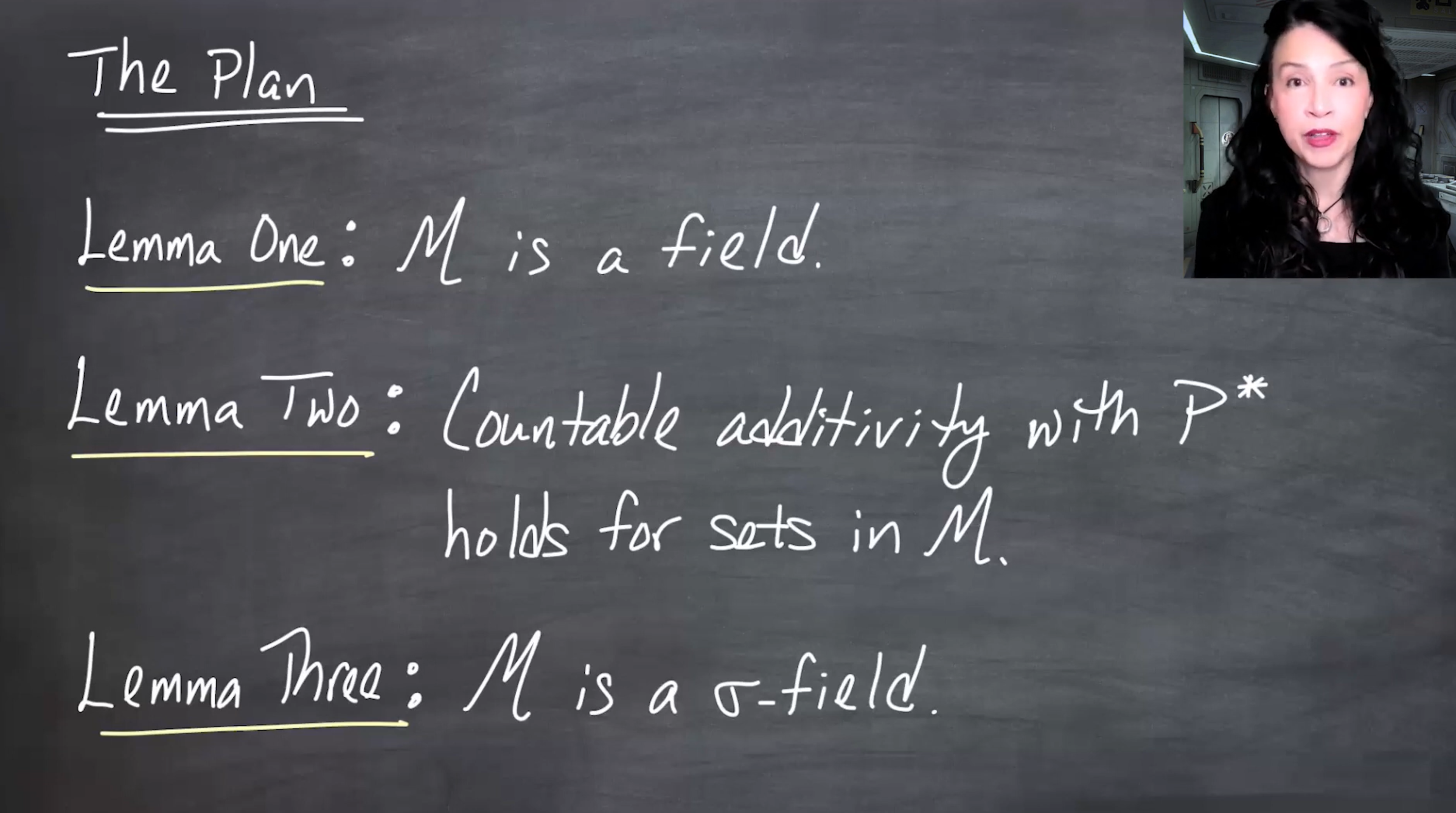
150.8.1 Lemma 1

\mathcal{M} \text{ is a field.}

This means:

1. \Omega\in\mathcal{M};
2. if A\in\mathcal{M}, then A^c\in\mathcal{M};
3. if A,C\in\mathcal{M}, then A\cup C\in\mathcal{M}.

150.8.2 Lemma 2

P^* is countably additive on disjoint sets in \mathcal{M}:

P^*\left(\bigcup_{n=1}^{\infty}A_n\right) = \sum_{n=1}^{\infty}P^*(A_n),

whenever A_1,A_2,\ldots\in\mathcal{M} are disjoint.

150.8.3 Lemma 3

\mathcal{M} \text{ is a } \sigma\text{-field.}

Lemma 2 helps upgrade finite-union closure to countable-union closure.

Lemma roadmap, second half.

Figure 150.11: The next three lemmas connect the new class \mathcal{M} back to the original field \mathcal{F}_0 and prove that P^* really extends P.

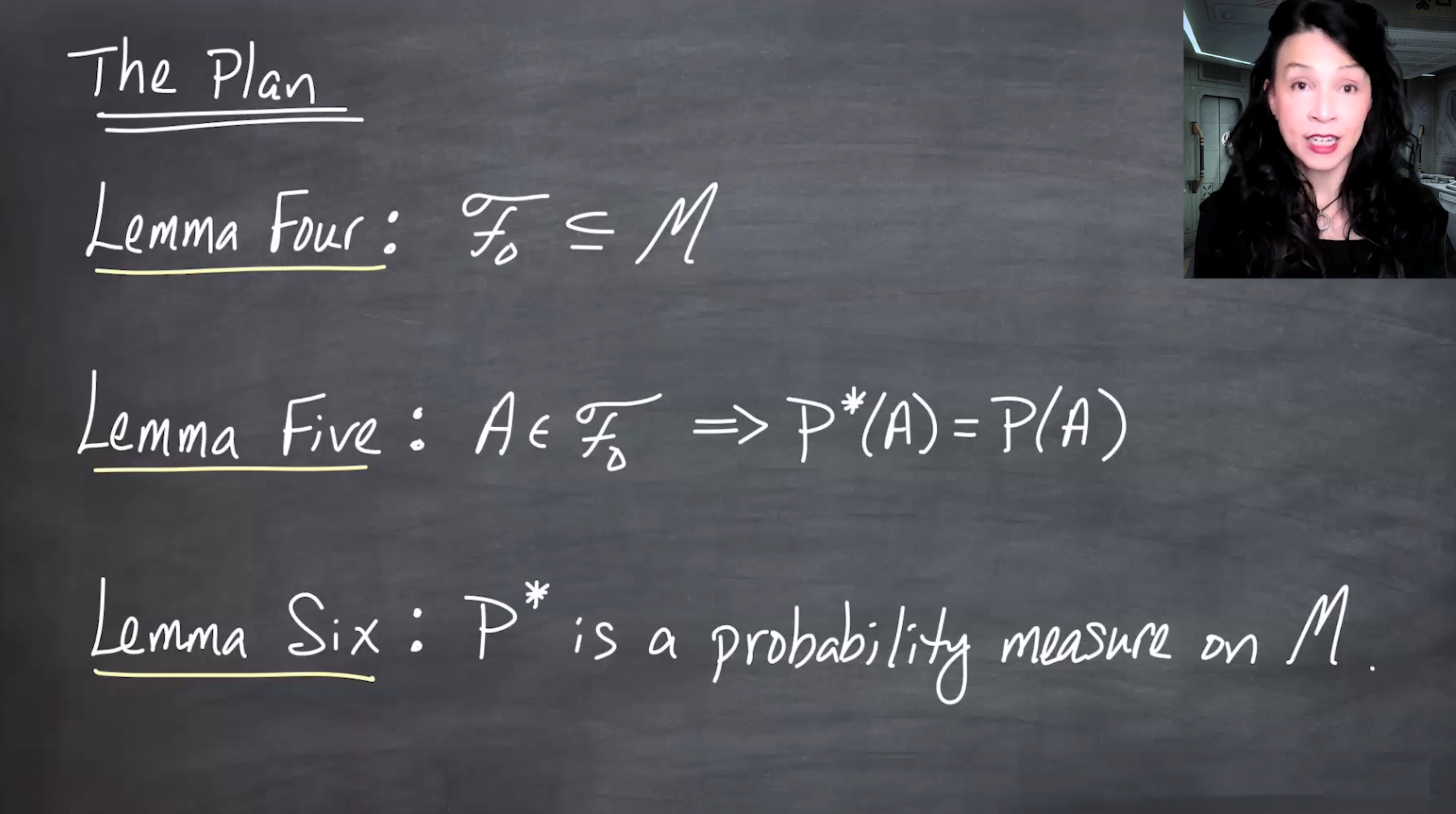
150.8.4 Lemma 4

\mathcal{F}_0\subseteq\mathcal{M}.

Every original field set satisfies the splitting condition.

150.8.5 Lemma 5

For every A\in\mathcal{F}_0,

P^*(A)=P(A).

This completes the equality that Lesson 4 only proved in one direction.

150.8.6 Lemma 6

P^* is a probability measure on \mathcal{M}.

That is:

1. P^*(\emptyset)=0;
2. P^* is countably additive on \mathcal{M};
3. P^*(\Omega)=1.

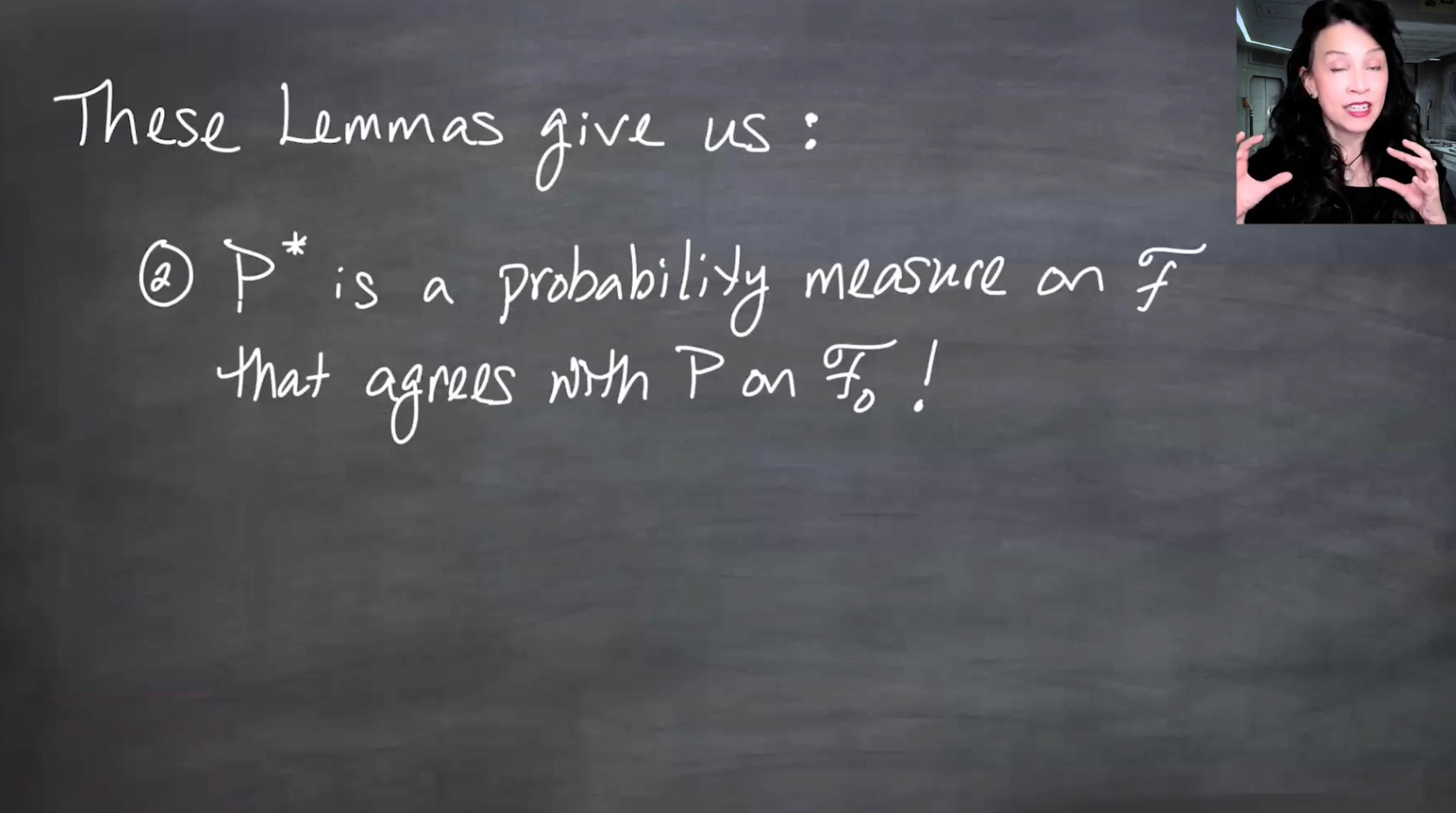
150.9 How the lemmas prove the extension theorem

Once the six lemmas are known, the extension theorem follows quickly.

Since Lemma 3 says \mathcal{M} is a \sigma-field, and Lemma 4 says \mathcal{F}_0\subseteq\mathcal{M}, the generated \sigma-field must satisfy

\mathcal{F} = \sigma(\mathcal{F}_0) \subseteq \mathcal{M}.

This is the same minimality argument used earlier: \sigma(\mathcal{F}_0) is the smallest \sigma-field containing \mathcal{F}_0, so it must be contained in any \sigma-field that contains \mathcal{F}_0.

The generated sigma-field is sandwiched between F naught and M.

Figure 150.12: The key containment is \mathcal{F}_0\subseteq\mathcal{F}\subseteq\mathcal{M}. This puts the target \sigma-field inside the class where P^* is already known to be a probability measure.

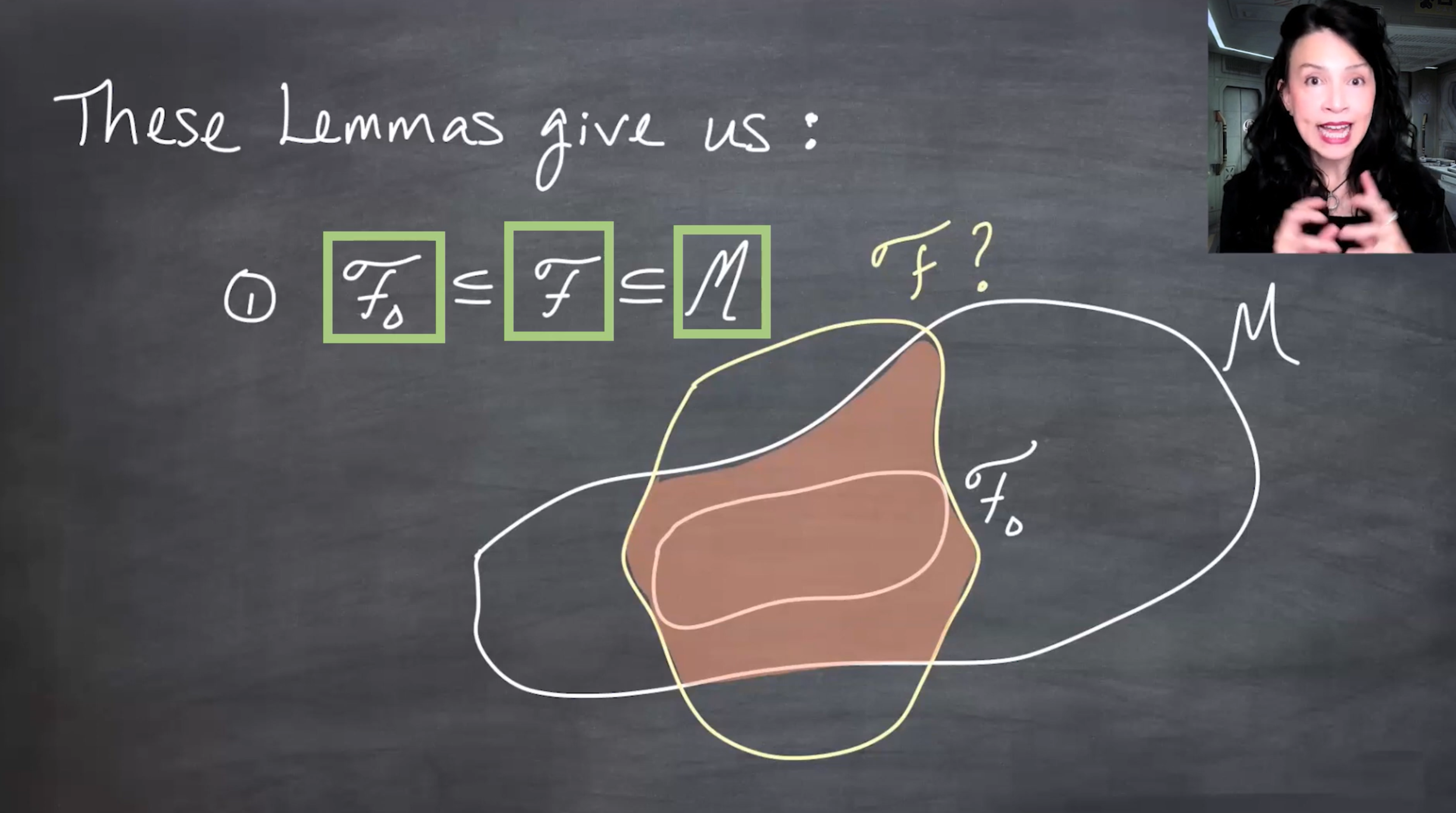
Since P^* is a probability measure on \mathcal{M}, it is also a probability measure when restricted to the smaller \sigma-field \mathcal{F}.

And since Lemma 5 says P^*=P on \mathcal{F}_0, this restriction is an extension of the original probability measure.

P star becomes a probability measure on the generated sigma-field.

Figure 150.13: The conclusion is the desired extension: P^* is a probability measure on \mathcal{F}=\sigma(\mathcal{F}_0) and agrees with P on the original field \mathcal{F}_0.

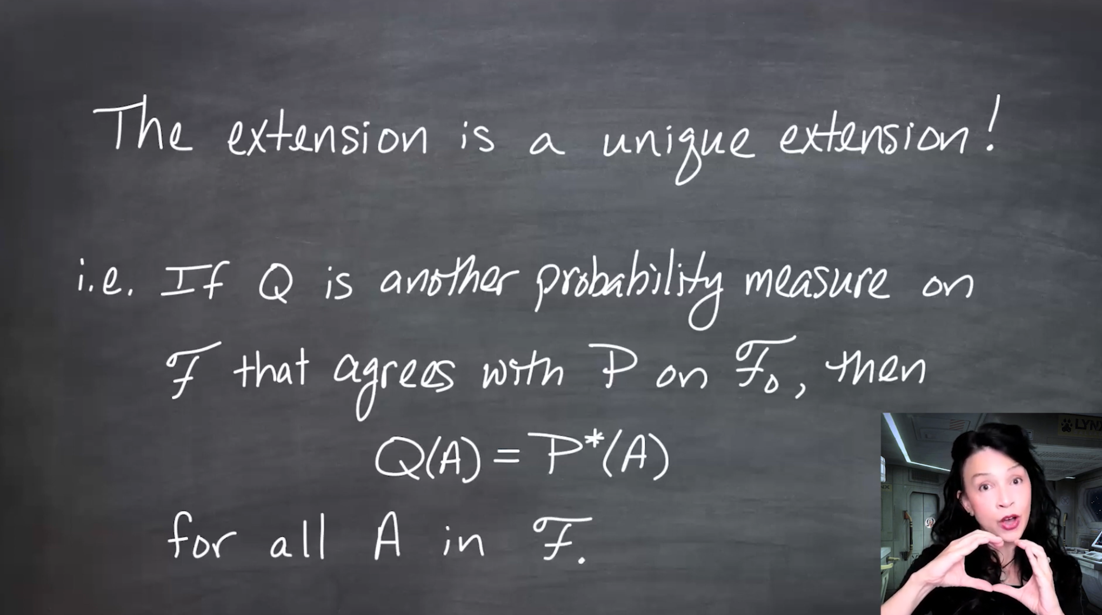
150.10 Uniqueness of the extension

The lesson also proves a uniqueness result.

Suppose Q is another probability measure on \mathcal{F} and Q agrees with P on \mathcal{F}_0:

Q(A)=P(A) \qquad \text{for all } A\in\mathcal{F}_0.

Then

Q(A)=P^*(A) \qquad \text{for all } A\in\mathcal{F}.

Uniqueness statement for the extension.

Figure 150.14: The extension is unique among probability measures on \mathcal{F} that agree with the original P on \mathcal{F}_0.

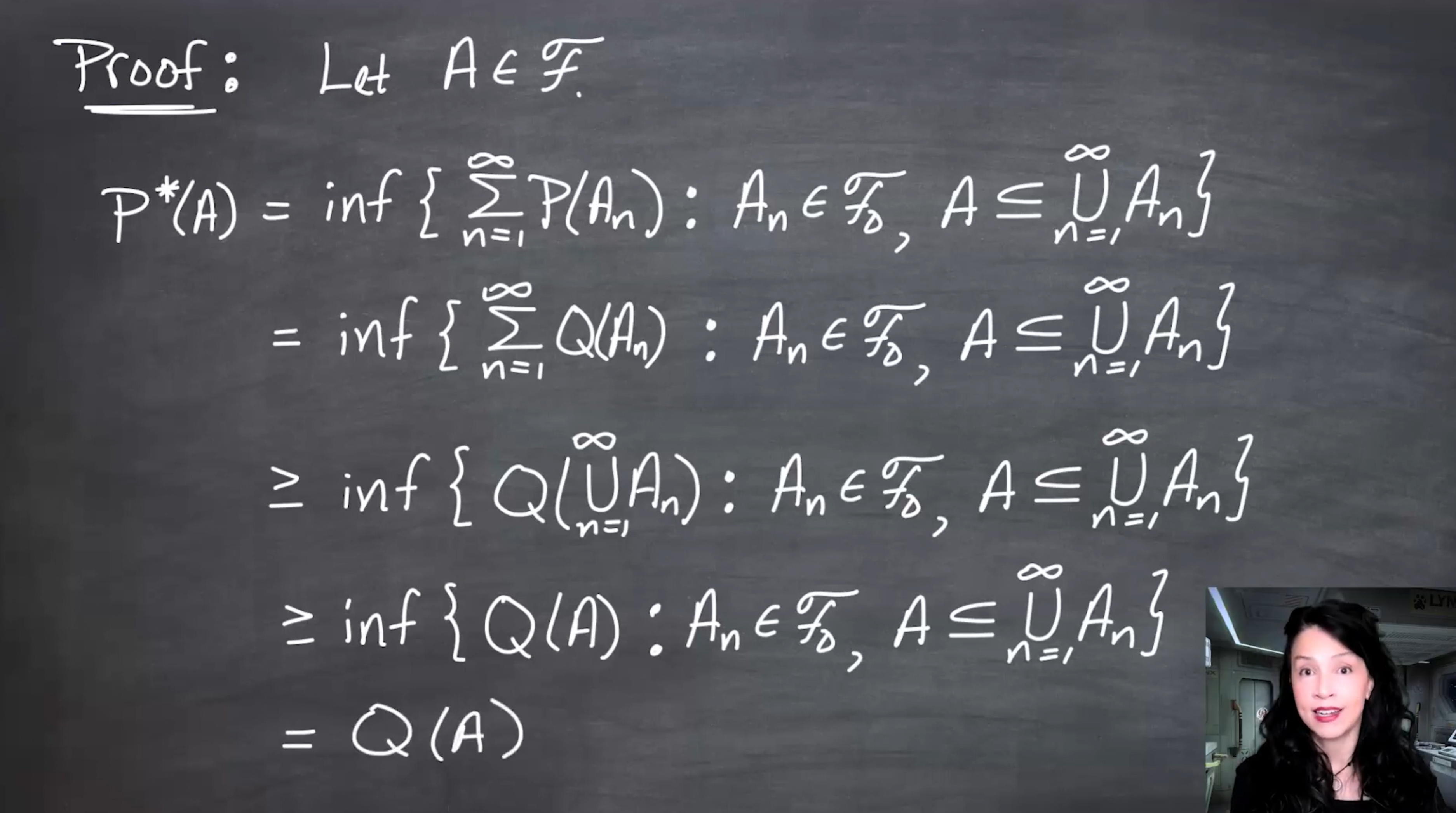
150.10.1 First inequality

Take A\in\mathcal{F}. By definition,

P^*(A) = \inf \left\{ \sum_{n=1}^{\infty}P(A_n) : A_n\in\mathcal{F}_0,\; A\subseteq\bigcup_n A_n \right\}.

Since Q=P on \mathcal{F}_0,

P^*(A) = \inf \left\{ \sum_{n=1}^{\infty}Q(A_n) : A_n\in\mathcal{F}_0,\; A\subseteq\bigcup_n A_n \right\}.

By countable subadditivity of Q,

Q\left(\bigcup_n A_n\right) \leq \sum_n Q(A_n).

And since A\subseteq\bigcup_n A_n, monotonicity gives

Q(A) \leq Q\left(\bigcup_n A_n\right).

Therefore every admissible cover-sum is at least Q(A), so

P^*(A)\geq Q(A).

First half of the uniqueness proof.

Figure 150.15: The cover-sums defining P^*(A) are all at least Q(A), so their infimum is also at least Q(A).

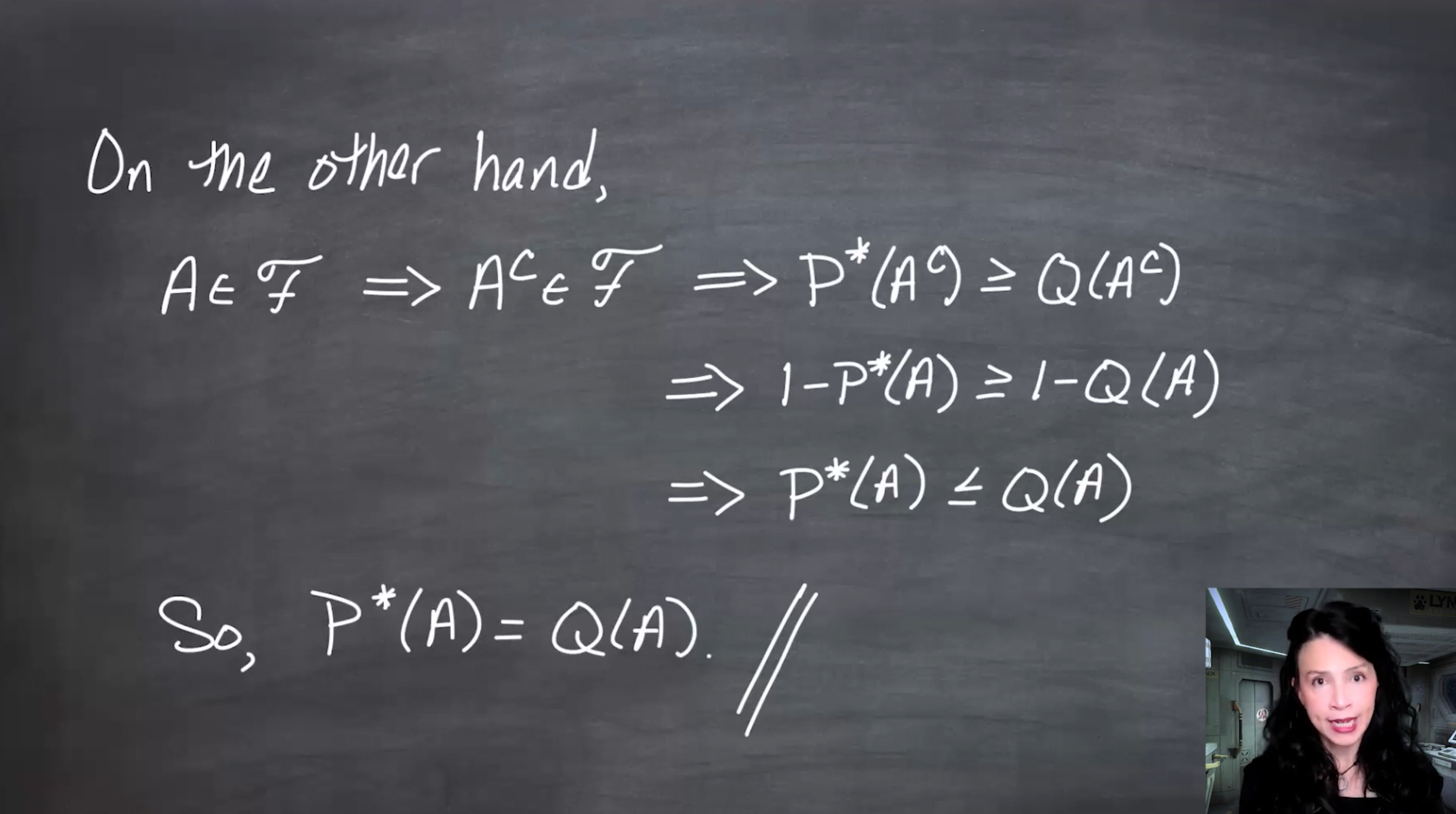
150.10.2 Reverse inequality

Since A\in\mathcal{F}, also A^c\in\mathcal{F}. Applying the previous inequality to A^c gives

P^*(A^c)\geq Q(A^c).

Both P^* and Q are probability measures on \mathcal{F}, so

P^*(A^c)=1-P^*(A), \qquad Q(A^c)=1-Q(A).

Thus,

1-P^*(A)\geq 1-Q(A),

which implies

P^*(A)\leq Q(A).

Combining both inequalities,

P^*(A)=Q(A).

Second half of the uniqueness proof using complements.

Figure 150.16: The complement trick turns the first inequality around. Together, the two inequalities force P^*(A)=Q(A).

150.11 Stronger uniqueness theorem

The lesson ends by noting a stronger result:

If P_1 and P_2 are probability measures on \mathcal{F}=\sigma(\mathcal{F}_0) and

P_1(A)=P_2(A) \qquad \text{for all } A\in\mathcal{F}_0,

then

P_1(A)=P_2(A) \qquad \text{for all } A\in\mathcal{F}.

This stronger theorem does not depend on the outer-measure definition of P^*.

A stronger uniqueness theorem for probability measures.

Figure 150.17: Agreement on the generating field determines the probability measure on the generated \sigma-field.

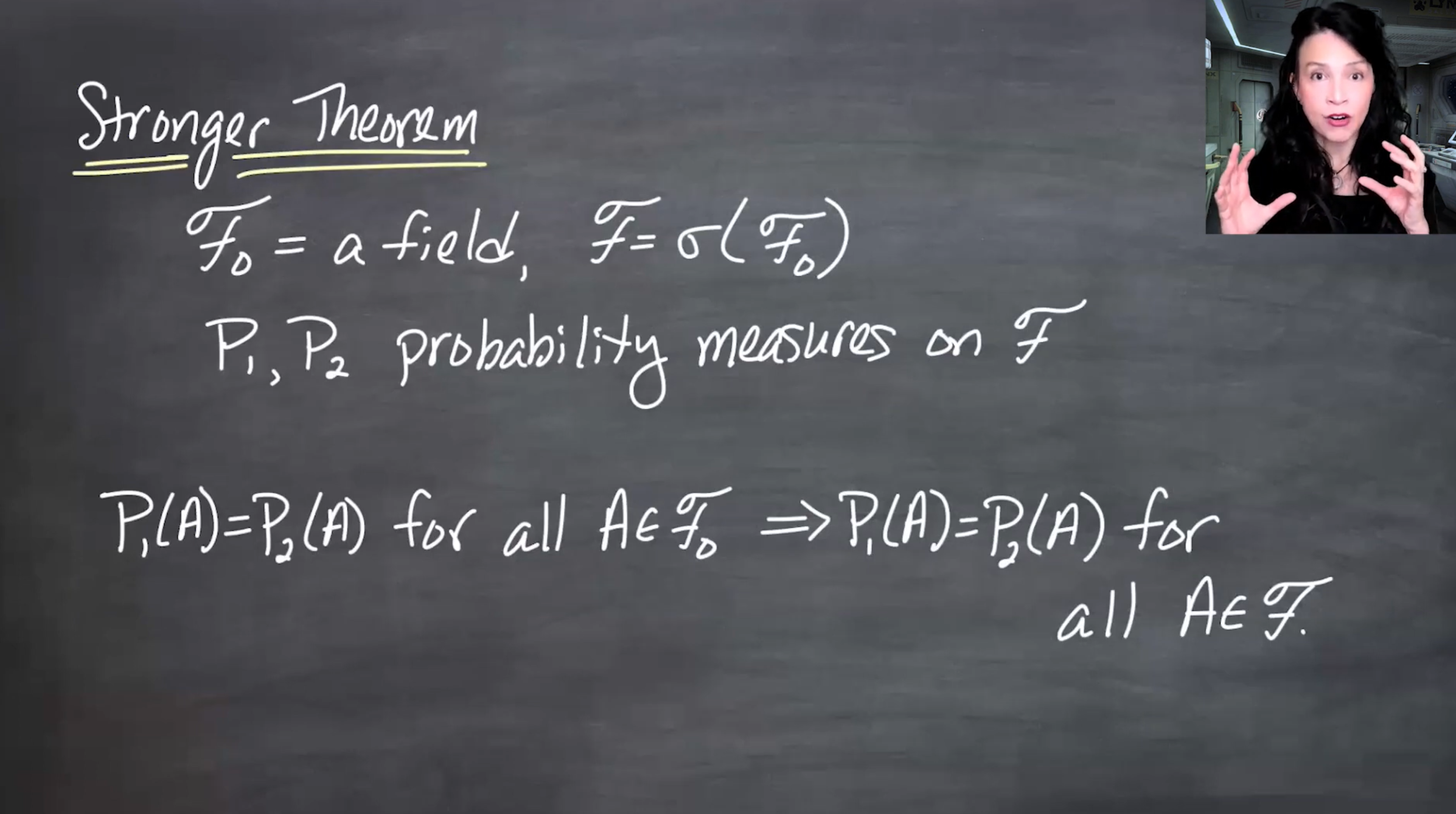
Jen notes that this stronger result is often proved using a weaker structure than a field, called a \pi-system, which will appear later.

Reference to stronger results using pi-systems.

Figure 150.18: A \pi-system is closed under finite intersections and is weaker than a field. It is enough for many uniqueness theorems for probability measures.

150.12 Takeaway

The outer measure P^* is a “wannabe probability measure.” It is defined on all subsets of \Omega, but it becomes a genuine probability measure only on the right class of measurable sets.

The proof strategy is:

P \text{ on } \mathcal{F}_0 \quad\longrightarrow\quad P^* \text{ on all subsets of } \Omega \quad\longrightarrow\quad \mathcal{M} \text{ where } P^* \text{ behaves additively} \quad\longrightarrow\quad P^* \text{ on } \sigma(\mathcal{F}_0).

The six lemmas are the scaffolding that turns the outer-measure construction into a true extension theorem.