124.1 What is a state-space model and why do I need to know about them
124.1.1 Example of a continuous-time state-space model
- Representation of the dynamics of an nth-order system as a first-order differential equation in an n-vector called the state.
- n coupled first-order equations.
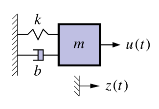
- Classic example: Second-order equation of motion
\begin{aligned} m\ddot{z}(t) &= u(t) - b \dot{z}(t) -k z(t) \\ \ddot{z}(t) &= \frac{1}{m} u(t) - \frac{b}{m} \dot{z}(t) -\frac{k}{m} z(t) \\ \end{aligned} \tag{124.1}
- where:
- m is the mass,
- z(t) is the position of the mass at time t,
- \dot{z}(t)= \frac{d z(t)}{dt} is the velocity of the mass at time t,
- \ddot{z}(t) = \frac{d^2 z(t)}{dt^2} is the acceleration of the mass at time t,
- k is the spring constant,
- b is the damping coefficient,
- Define a (non-unique) state vector:
x(t) = \begin{bmatrix} z(t) \\ \dot{z}(t) \end{bmatrix}, \quad \therefore \quad \dot{x}(t) = \begin{bmatrix} \dot{z}(t) \\ \ddot{z}(t) \end{bmatrix} = \begin{bmatrix} \dot{z}(t) \\ \frac{u(t) - b \dot{z}(t) - kz(t)}{m} \end{bmatrix}
124.1.2 Example in continuous-time state-space form
- So far, we have:
\dot{x}(t) = \begin{bmatrix} z(t) \\ \dot{z}(t) \end{bmatrix} = \begin{bmatrix} \dot{z}(t) \\ \frac{u(t) - b \dot{z}(t) - kz(t)}{m} \end{bmatrix}
- We can rewrite this as \dot{x}(t) = Ax(t) + Bu(t) where A and B are constant matrices.
\dot{x}(t) = \begin{bmatrix} z(t) \\ \dot{z}(t) \end{bmatrix} = \underbrace{\begin{bmatrix} \phantom{0} & \phantom{0} \\ \phantom{0} & \phantom{0}\end{bmatrix}}_{A} x(t) + \underbrace{\begin{bmatrix} \phantom{0} & \phantom{0} \\ \phantom{0} & \phantom{0} \end{bmatrix}}_{B} u(t)
- Complete the model by computing z(t) = Cx(t) + Du(t) where C and D are constant matrices.
C = \begin{bmatrix} \phantom{0} & \phantom{0} \\ \phantom{0} & \phantom{0} \end{bmatrix} \qquad D = \begin{bmatrix} \phantom{0} & \phantom{0} \\ \phantom{0} & \phantom{0} \end{bmatrix}
124.1.3 Standard state-space model form
- Standard form for continuous-time linear state-space model:
\begin{aligned} \dot{x}(t) &= Ax(t) + Bu(t) + w(t) \\ z(t) &= Cx(t) + Du(t) + v(t) \end{aligned} \tag{124.2}
- where
- u(t) is the known input,
- x(t) is the state,
- A, B, C, D are constant matrices.
- Convenient way to express dynamics (matrix format great for computers).
- The first equation is called the state equation or the process equation.
- Note that this is the only equation that evolves over time (since it is a first-order vector ODE that integrates the right-hand side to find x(t)).
- So, this equation summarizes the dynamics of the model.
- The second equation is called the output equation or the measurement equation.
- It is a static linear combination of variables known at time t.
124.1.4 What is the system state vector?
- Standard form for continuous-time linear state-space model: \begin{aligned} \dot{x}(t) &= Ax(t) + Bu(t) + w(t) \\ z(t) &= Cx(t) + Du(t) + v(t) \end{aligned}
- We think of the system state at time t_0 as a minimum set of information at t_0 that, together with input u(t), t \ge t_0, uniquely determines system behavior for all t \ge t_0.
- State variables provide access to what is going on inside the system.
- The state has dimensions x(t) \in \mathbb{R}^n, so A \in \mathbb{R}^{n \times n} and w(t) \in \mathbb{R}^n.
- Note that in principle we can solve the state equation numerically,
x(t) = x(0) + \int_0^t A x(\tau) + B u(\tau) + w(\tau) d\tau \qquad (\text {integral form})
- but it will usually be more convenient to keep the equation in differential form.
124.1.5 What are the output and inputs?
- Standard form for continuous-time linear state-space model: \begin{aligned} \dot{x}(t) &= Ax(t) + Bu(t) + w(t) \\ z(t) &= Cx(t) + Du(t) + v(t) \end{aligned}
- The model output is z(t) \in \mathbb{R}^m. This is the measurement we make.
- There are three input signals to the model: u(t), w(t), and v(t).
- We consider u(t) \in \mathbb{R}^r to be a deterministic input, i.e. we we know its value exactly at all times.
- Based on the size of u(t), we infer that B \in \mathbb{R}^{n \times r}.
- The deterministic input causes x(t) to evolve over time in different ways, depending on its values.
- It also influences the output via the D term
124.1.6 What are the random (stochastic) inputs?
- Standard form for continuous-time linear state-space model: \begin{aligned} \dot{x}(t) &= Ax(t) + Bu(t) + w(t) \\ z(t) &= Cx(t) + Du(t) + v(t) \end{aligned}
- The model has two random input signals: w(t) and v(t).
- They are random in the sense that we assume that we never know their values exactly.
- We have already seen that w(t) \in \mathbb{R}^n; if z(t) \in \mathbb{R}^m, then v(t) \in \mathbb{R}^m also.
- The w(t) signal is process noise. Note that it affects the dynamics of the model by making direct changes to the evolution of x(t).
- The v(t) signal is sensor noise. Note that it does not affect the dynamics of the model; it only affects the measurement z(t).
- Systems having noise inputs w(t) and v(t) are considered in detail in week 3
124.1.7 What are the matrices called?
- Standard form for continuous-time linear state-space model: \begin{aligned} \dot{x}(t) &= Ax(t) + Bu(t) + w(t) \\ z(t) &= Cx(t) + Du(t) + v(t) \end{aligned} \tag{124.3}
- A \in \mathbb{R}^{n \times n} is the system matrix which models the evolution of the state in the absence of input.
- B \in \mathbb{R}^{n \times r} is the input matrix which defines how linear combinations of u(t) impact the evolution of the state.
- C \in \mathbb{R}^{m \times n} is the output matrix which defines how the output depends on linear combinations of states.
- D \in \mathbb{R}^{m \times r} is the feed–forward or feed–through) matrix which models how the output depends on linear combinations of the input (instantaneously).
- Time-varying systems have A, B, C, D that change with time.
124.1.8 Why do you need to know about them?
- It can be of vital interest to know the state of the system, but we usually cannot measure it directly.
- Instead, we can measure u(t) and z(t), and although we cannot measure the random signals w(t) and v(t), we can model some of their critical attributes.
- This enables us to make methods to estimate x(t) based on what we measure and what we model.
- Kalman filters are (in some cases optimal) estimators of x(t)
- The derivation and implementation of the KF depends on modeling the system in state-space form and having knowledge of the model A, B, C, and D matrices.
- This is why we care!
124.1.9 Summary
State-space models are a compact representation of an nth-order linear system in terms of a 1st-order vector ODE.
The standard form for linear continuous-time state-space models is Equation 124.3
We have learned the names of the equations, the names of the matrices, and the names of the signals (and what they all mean).
We have seen one example of a model in state-space form;
Next, we shall look at three other important general models.