153.1 Lesson map
This lesson introduces limits of sequences of sets.
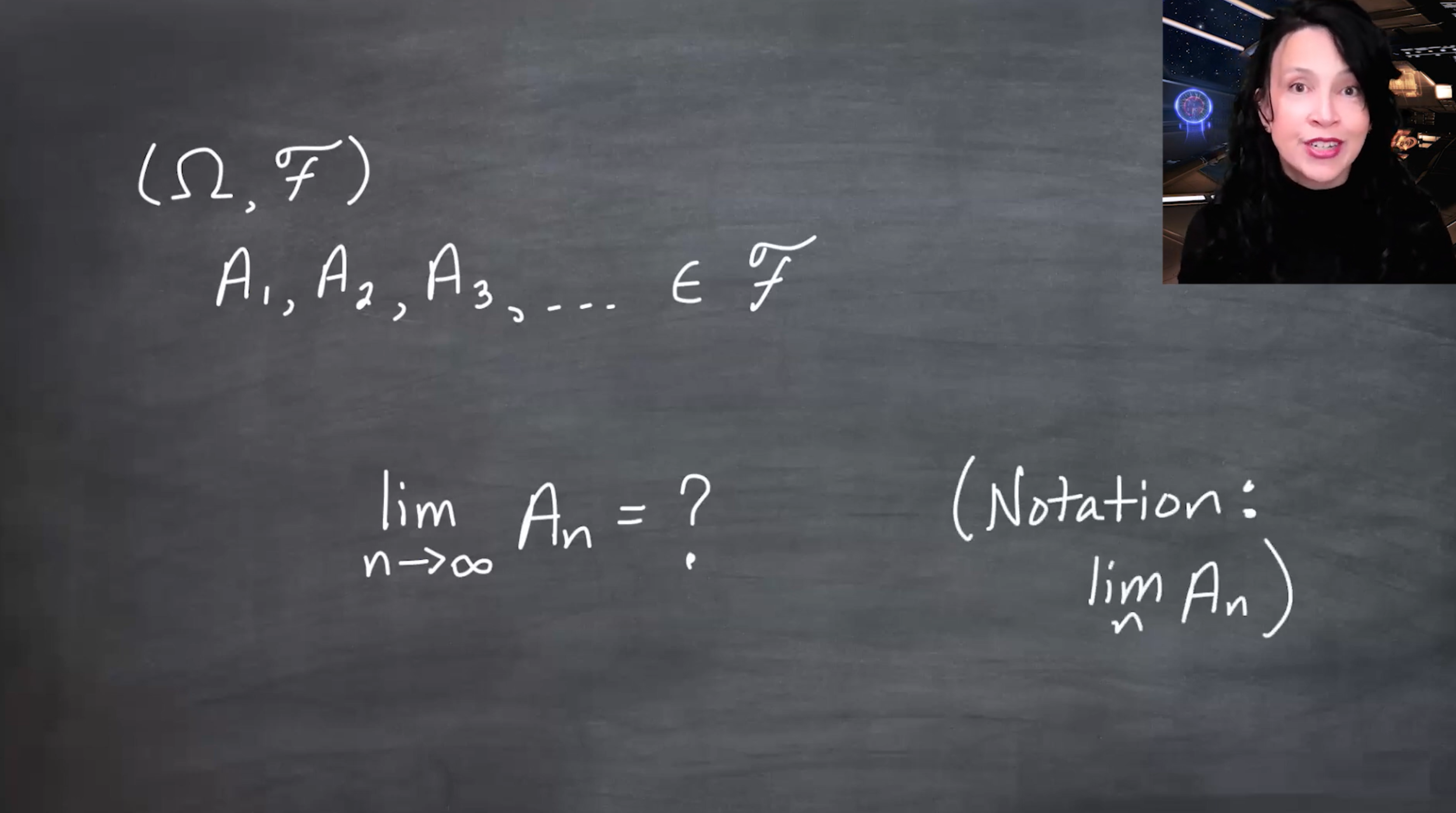
- 0:12 — What should \lim_n A_n mean for sets?
- 2:03 — First intuitive example: increasing intervals approaching [0,1).
- 3:24 — Review: \limsup and \liminf for sequences of real numbers.
- 10:29 — Decreasing sequences of sets: A_n\downarrow A.
- 12:06 — Increasing sequences of sets: A_n\uparrow A.
- 13:39 — General sequences: define \limsup A_n and \liminf A_n.
- 17:09 — Prove \liminf A_n\subseteq\limsup A_n.
- 19:35 — Define the limit of sets when \liminf A_n=\limsup A_n.
- 20:00 — Check decreasing sequences.
- 23:39 — Check increasing sequences.
- 24:18 — Revisit the interval example.
- 27:22 — Alternating-set example.
- 30:09 — Complements of \limsup and \liminf.
- 31:46 — Event interpretation: infinitely often and eventually.
- 34:09 — Measurability of \limsup A_n, \liminf A_n, and \lim A_n.
- 35:36 — Preview: continuity of probabilities.
153.2 Why limits of sets?
So far, collections like A_1,A_2,A_3,\ldots were mostly just indexed families. The order did not matter much when taking unions or intersections.
From now we begin to care about the order. How does the sequence of sets evolve over time - we might be dealing with a time series, their index being time. Or they may evolve so that an events may depend on a previous one. In any case, we want to understand the long-term behavior of a sequence of sets. A sequence of sets is meant to evolve: A_1, A_2, A_3, \ldots The question is whether this sequence has a limiting set.
153.3 First example: nested intervals
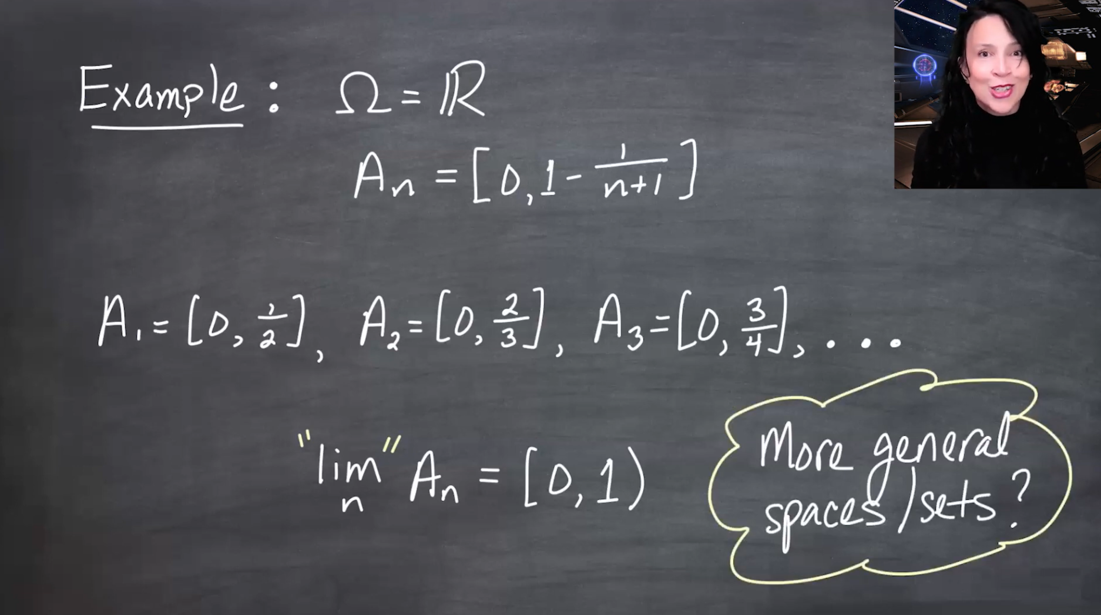
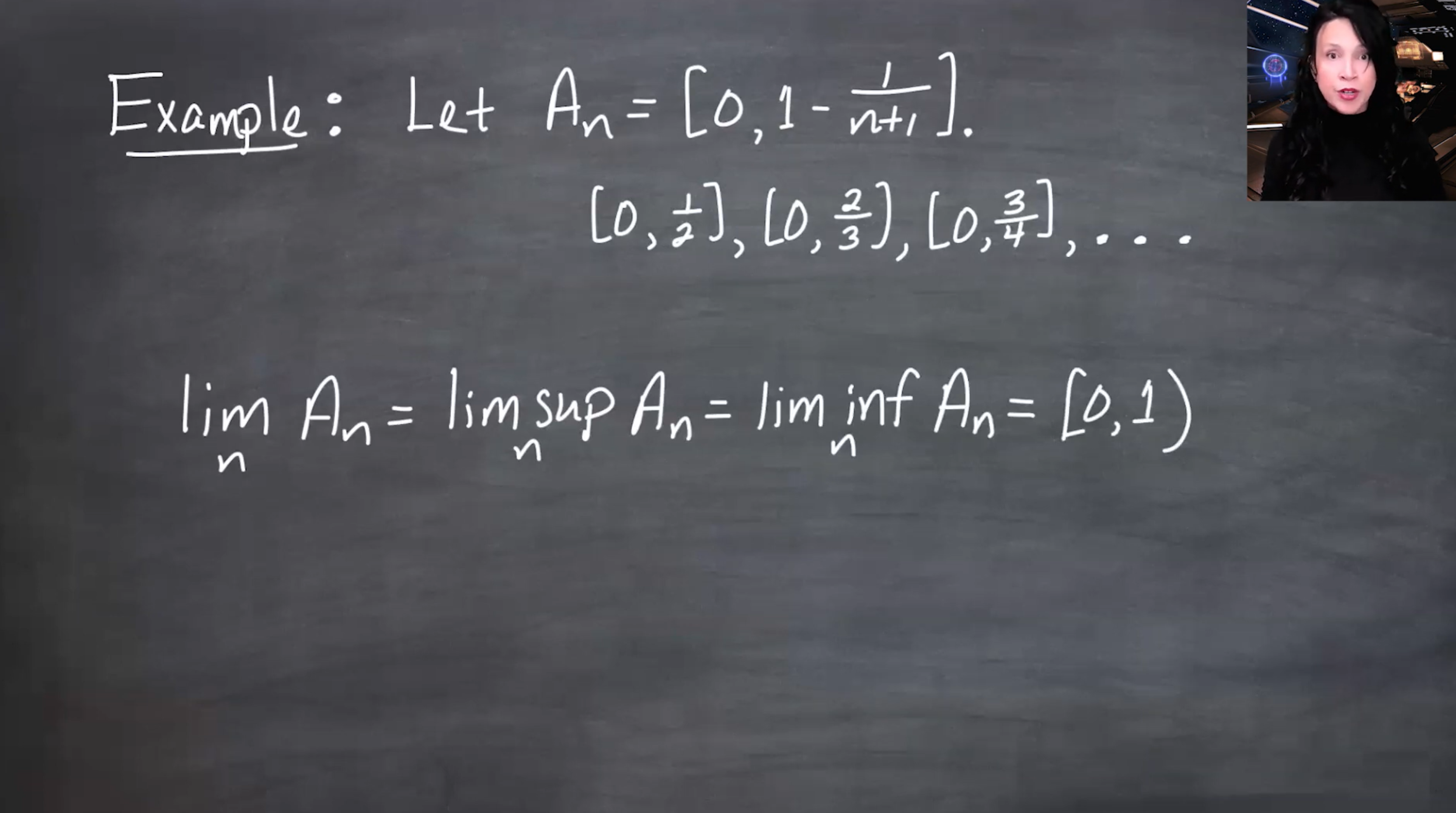
Let \Omega=\mathbb{R},\quad A_n=\left[0,1-\frac{1}{n+1}\right]. Then
A_1=\left[0,\frac12\right], \qquad A_2=\left[0,\frac23\right], \qquad A_3=\left[0,\frac34\right], \quad \ldots
The sets are increasing: A_1\subseteq A_2\subseteq A_3\subseteq\cdots., intuitively, they approach [0,1)
This example is geometrically clear, but we need a definition that also works for arbitrary measurable sets.
153.4 Warm-up: \limsup and \liminf of real sequences
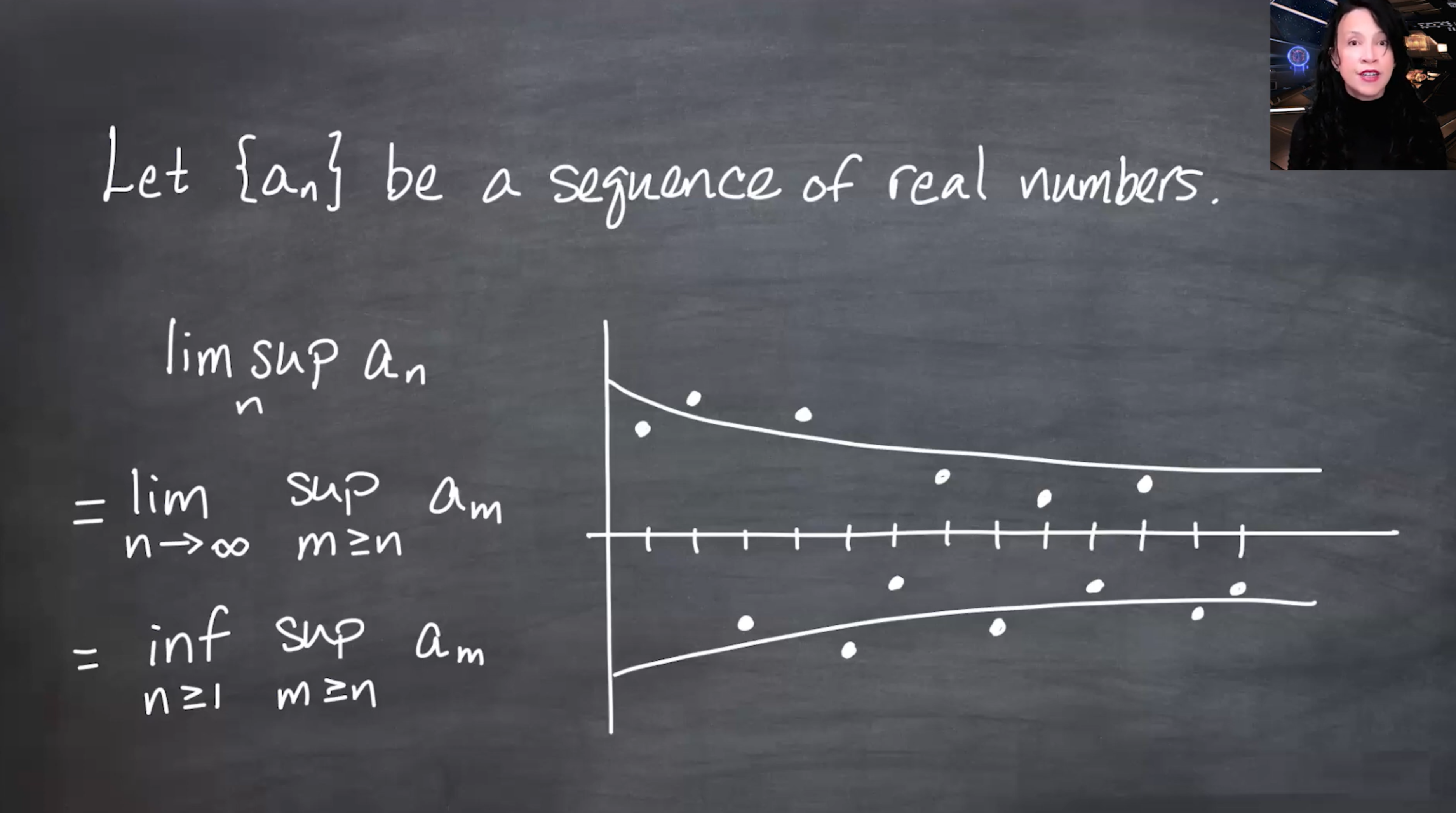
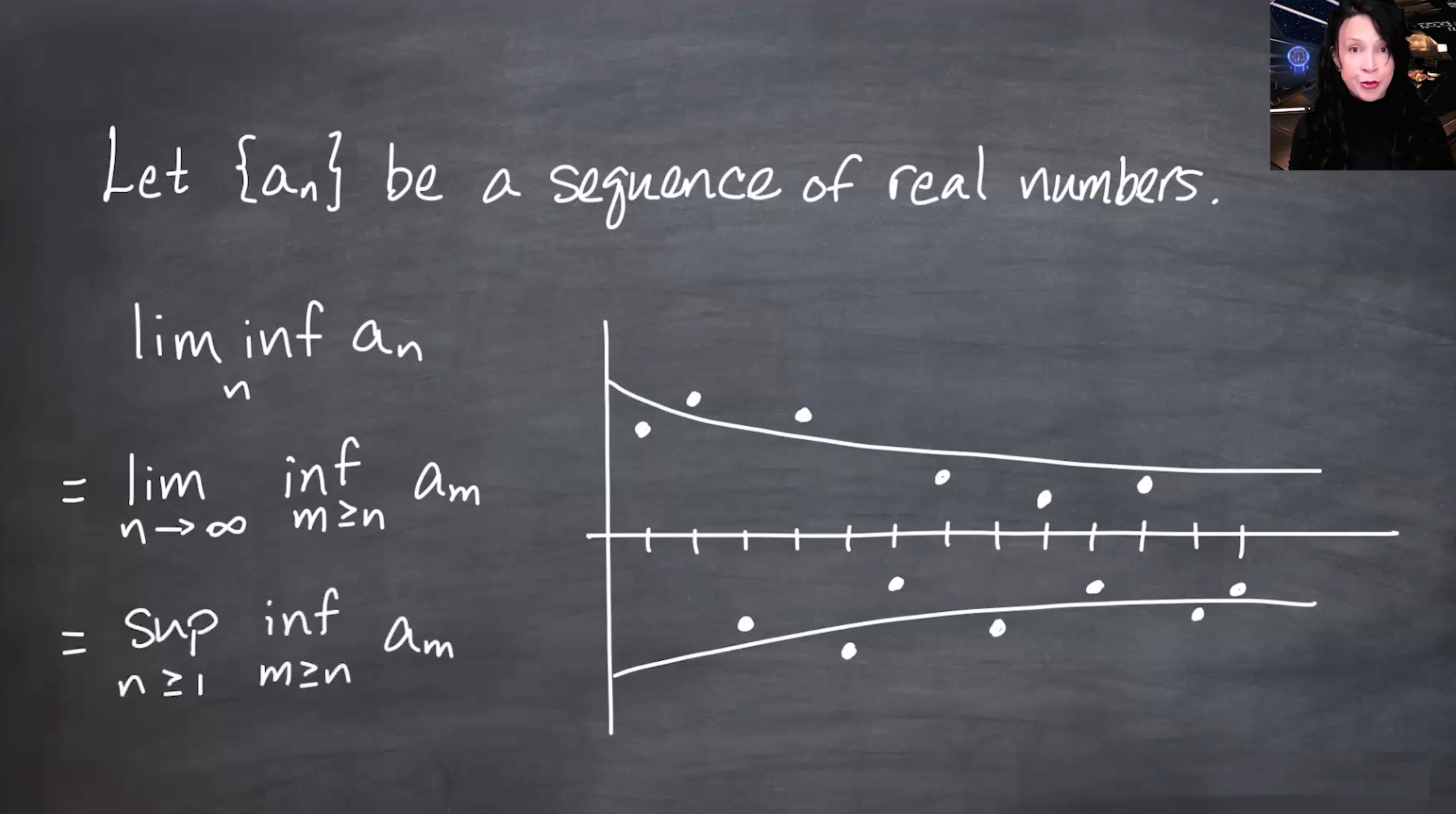
Before defining limits of sets, recall the analogous ideas for a real sequence a_1,a_2,a_3,\ldots. The limit superior or limit supremum tracks the eventual upper envelope of the sequence.
For each n, look at the tail \{a_m:m\geq n\}. Take the supremum of that tail: \sup_{m\geq n} a_m. As n increases, we discard more initial terms, so these tail suprema form a non-increasing sequence. The limit of these tail suprema is the \limsup:
\limsup_{n\to\infty} a_n = \lim_{n\to\infty} \sup_{m\geq n} a_m \tag{153.1}
Equivalently,
\limsup_{n\to\infty} a_n = \inf_{n\geq 1}\sup_{m\geq n}a_m. \tag{153.2}
Similarly, the limit inferior or limit infimum tracks the eventual lower envelope:
\liminf_{n\to\infty} a_n = \lim_{n\to\infty} \inf_{m\geq n}a_m = \sup_{n\geq 1}\inf_{m\geq n}a_m.
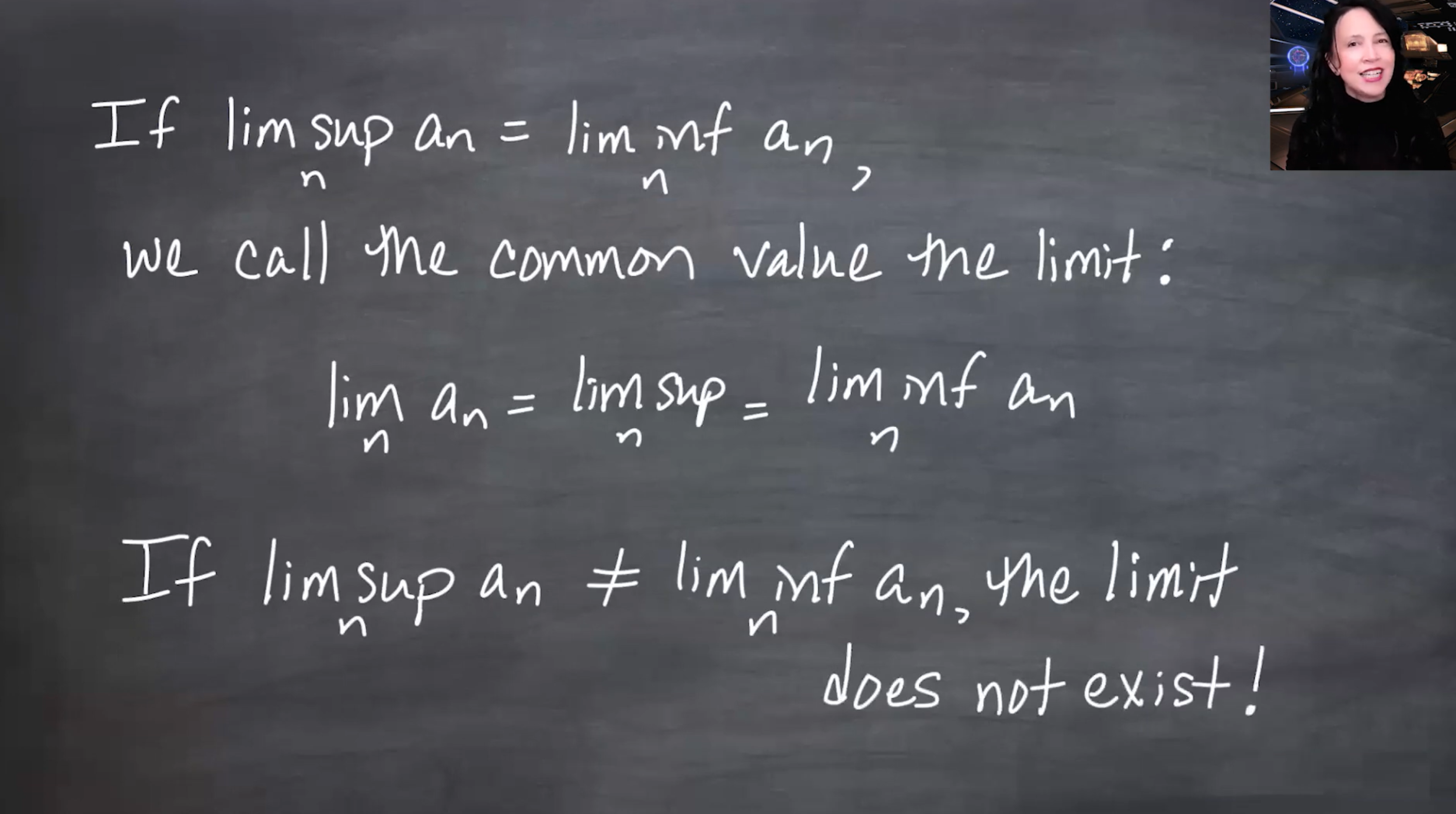
If the two envelopes meet, the sequence has a limit:
\limsup_{n\to\infty} a_n = \liminf_{n\to\infty} a_n = L.
Then
\lim_{n\to\infty} a_n=L.
The set version will imitate this idea, but with unions and intersections replacing suprema and infima.
153.5 Monotone sequences of sets
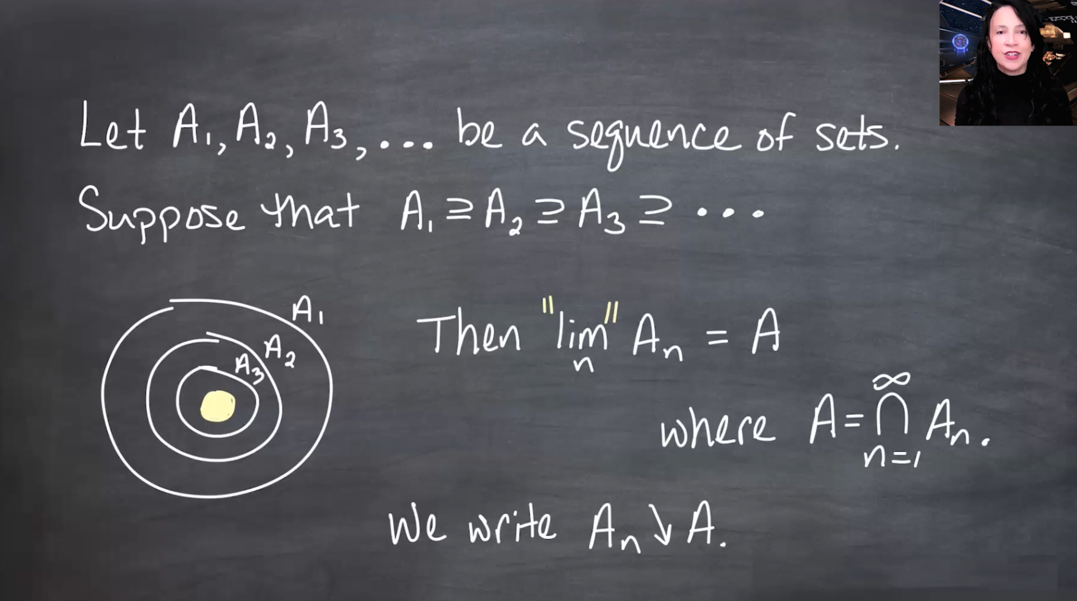
153.5.1 Decreasing sets
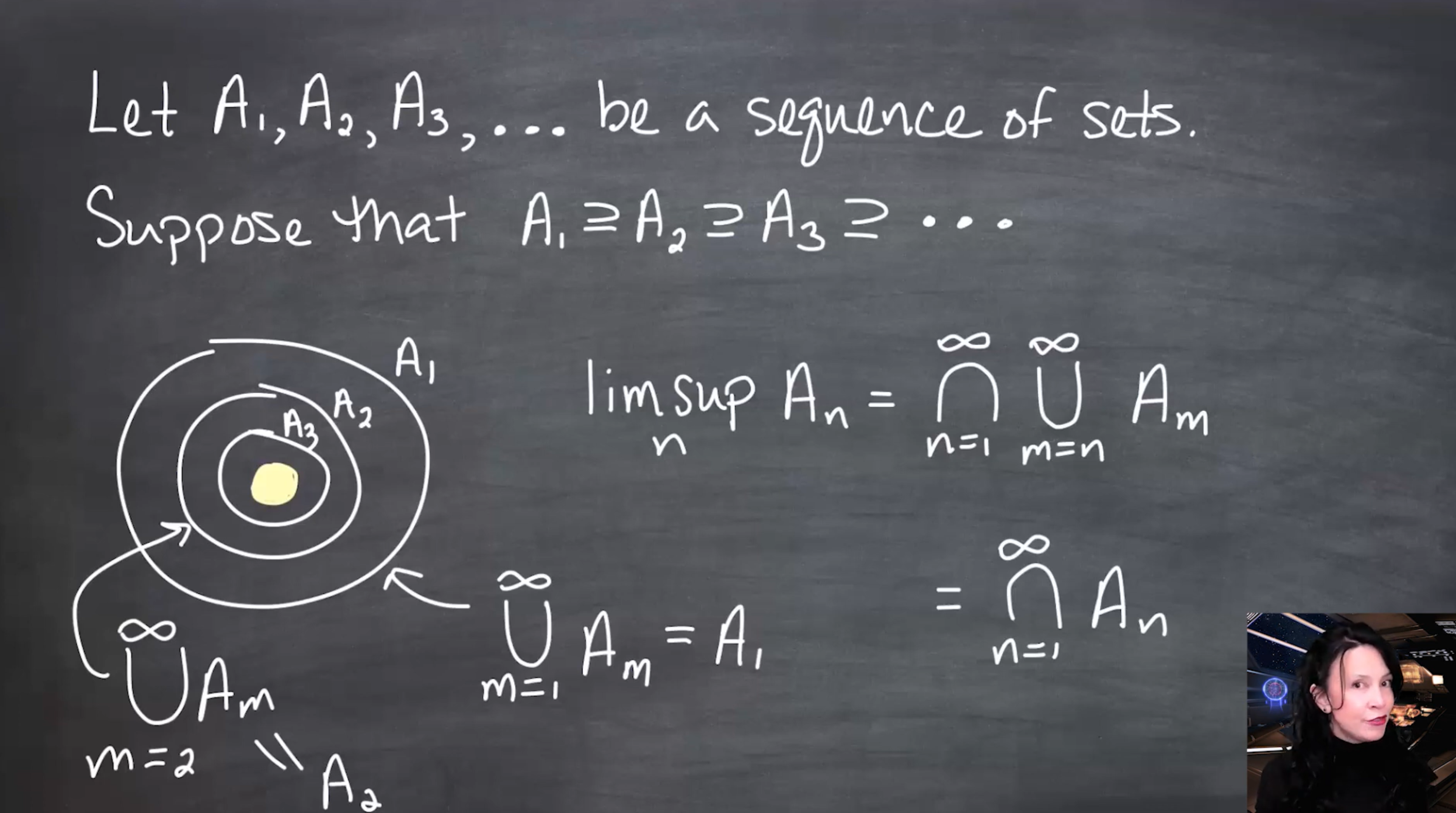
Suppose
A_1\supseteq A_2\supseteq A_3\supseteq\cdots.
Then the sets are decreasing. The natural limiting set is the part that remains forever:
A=\bigcap_{n=1}^{\infty}A_n.
We write
A_n\downarrow A.
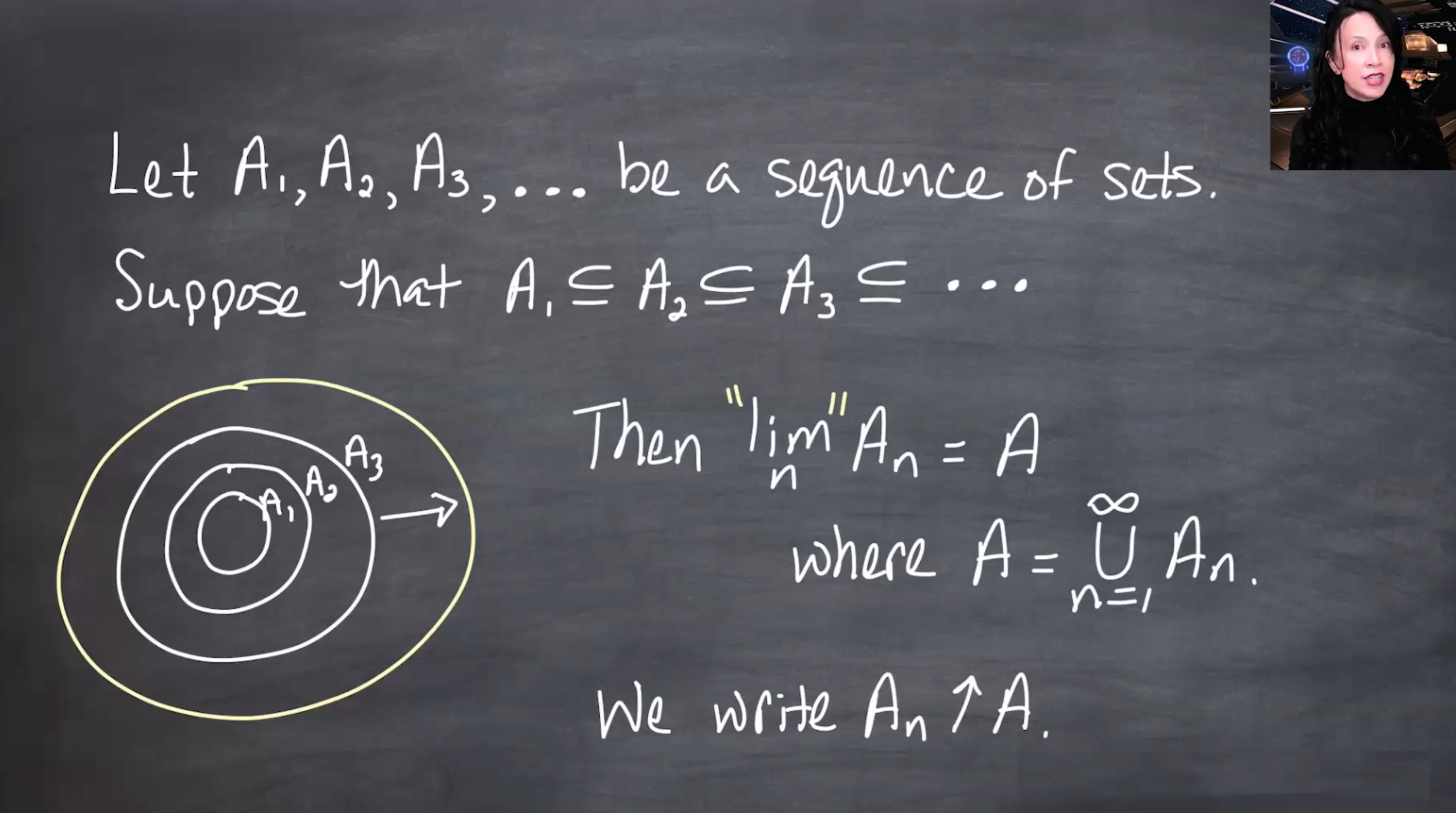
153.5.2 Increasing sets
Suppose
A_1\subseteq A_2\subseteq A_3\subseteq\cdots.
Then the sets are increasing. The natural limiting set is everything that eventually appears:
A=\bigcup_{n=1}^{\infty}A_n.
We write
A_n\uparrow A.
These two cases motivate the general definitions.
153.6 General sequences of sets
Now let
A_1,A_2,A_3,\ldots
be any sequence of sets. They need not be increasing, decreasing, disjoint, or nested.
To define the set-theoretic \limsup and \liminf, use tails of the sequence.
153.6.1 Tail unions
For each n, define the tail union
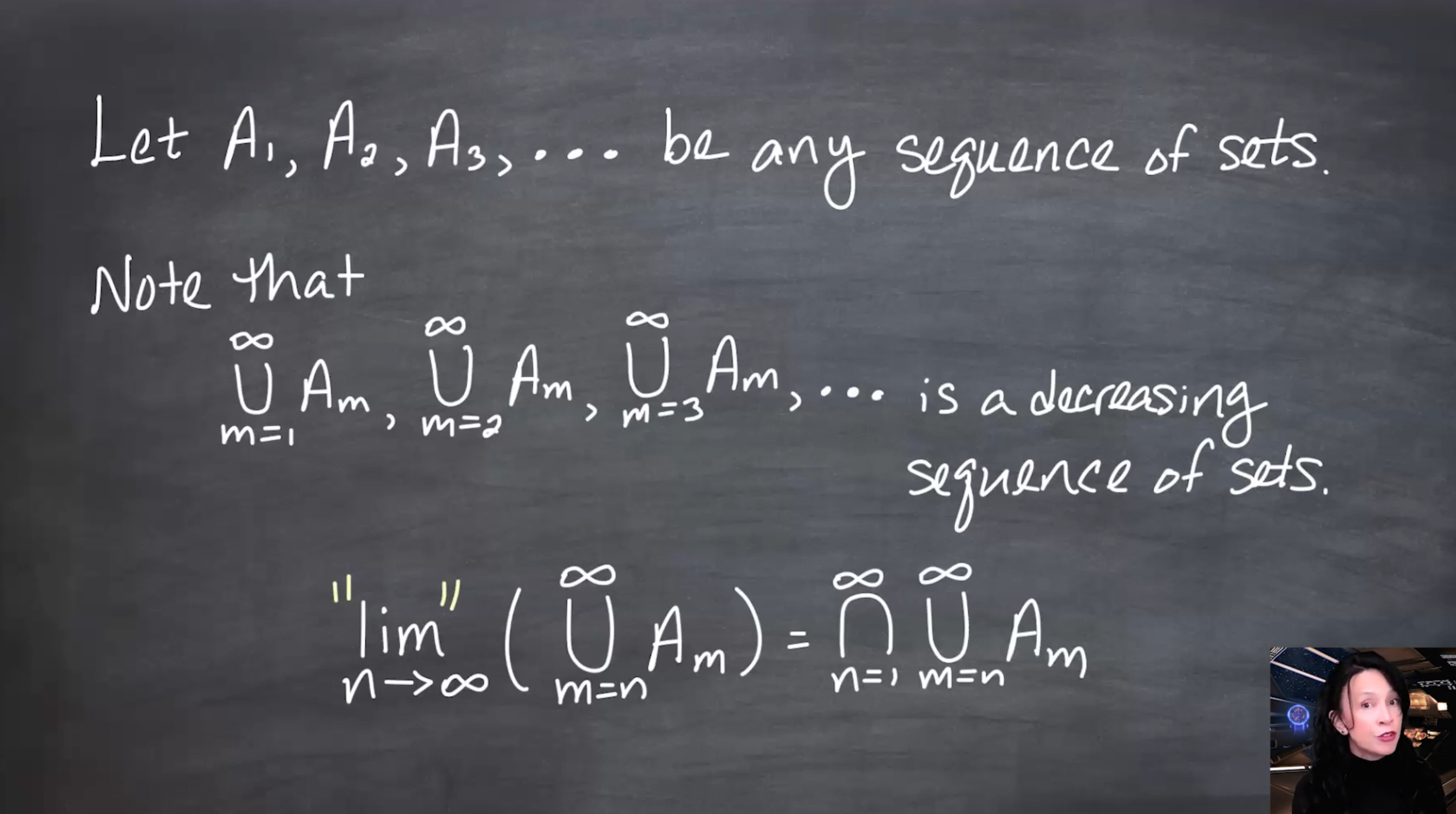
\bigcup_{m=n}^{\infty}A_m.
As n increases, we remove more initial sets, so the tail unions decrease:
\bigcup_{m=1}^{\infty}A_m \supseteq \bigcup_{m=2}^{\infty}A_m \supseteq \bigcup_{m=3}^{\infty}A_m \supseteq \cdots.
The limit of this decreasing sequence is its intersection.
153.6.2 Tail intersections
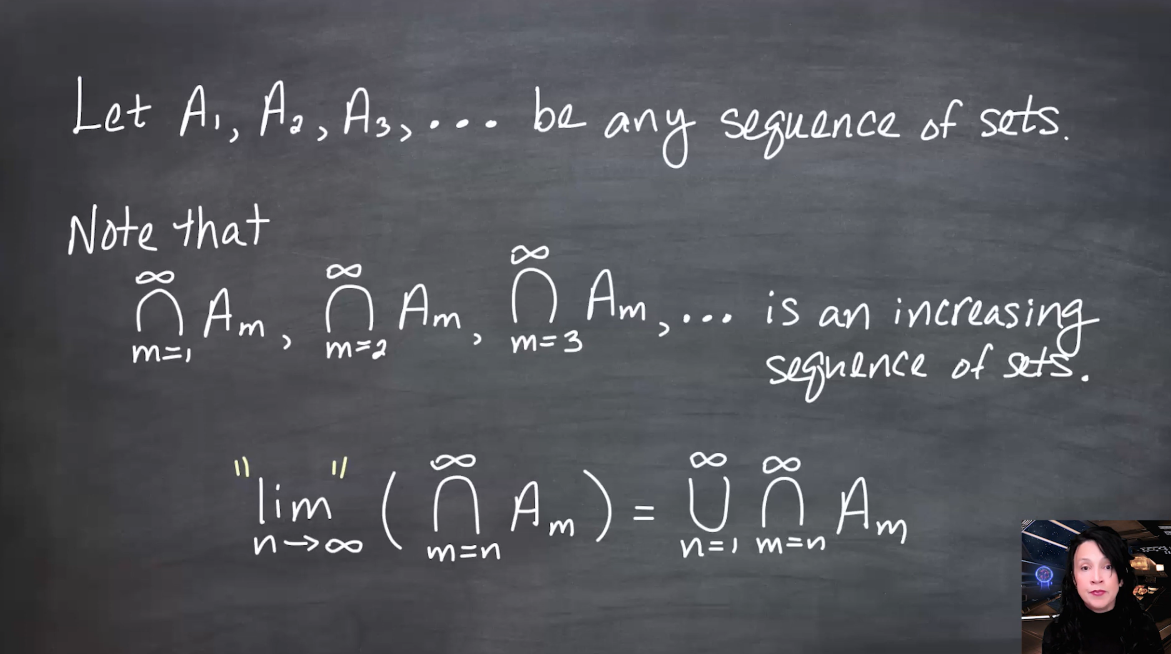
For each n, define the tail intersection
\bigcap_{m=n}^{\infty}A_m.
As n increases, we remove more initial constraints, so the tail intersections increase:
\bigcap_{m=1}^{\infty}A_m \subseteq \bigcap_{m=2}^{\infty}A_m \subseteq \bigcap_{m=3}^{\infty}A_m \subseteq \cdots.
The limit of this increasing sequence is its union.
153.7 Definitions: \limsup and \liminf of sets
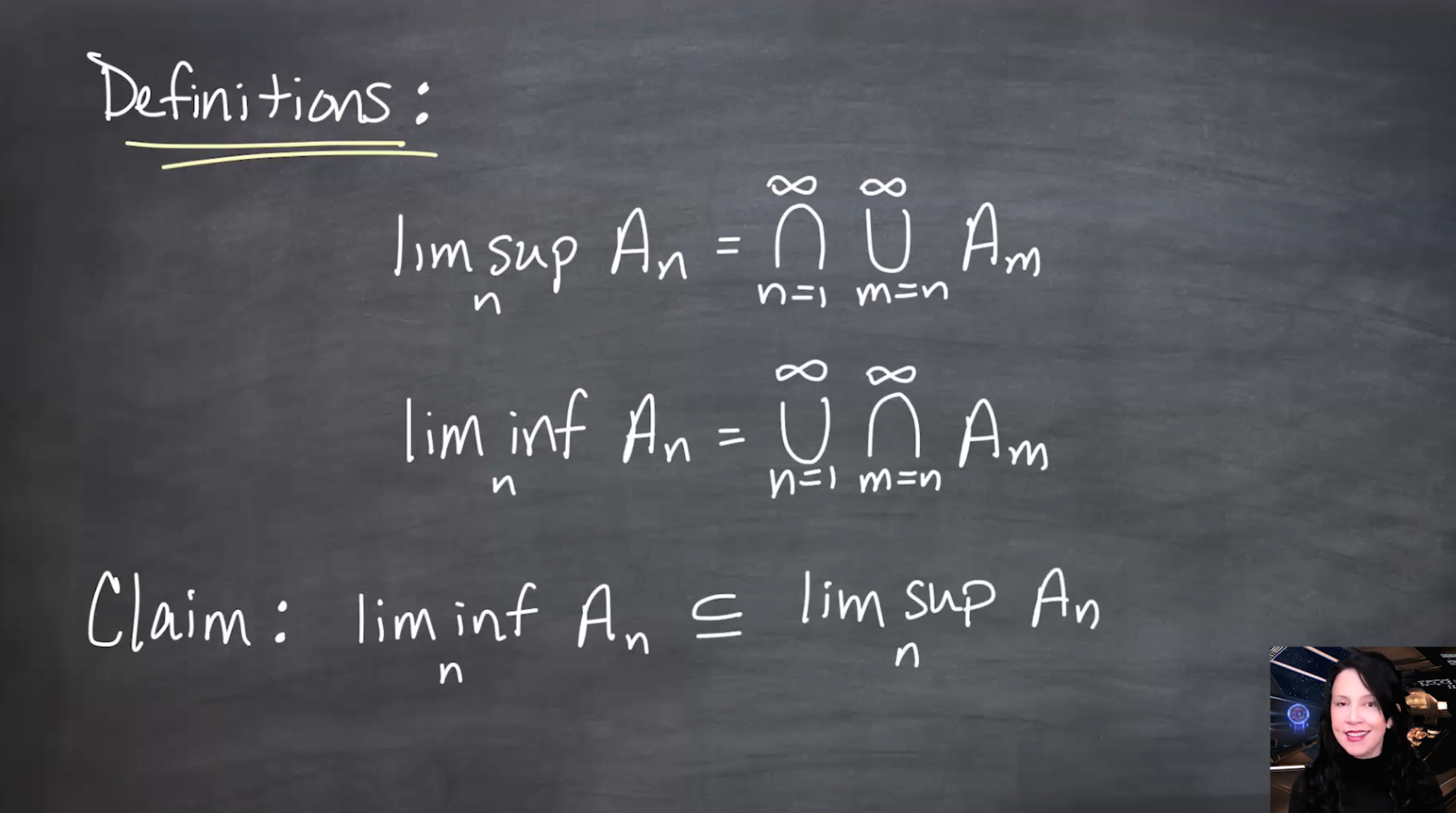
Definition 153.1 (Limit superior of sets) For a sequence of sets A_1,A_2,\ldots, define
\limsup_{n\to\infty} A_n = \bigcap_{n=1}^{\infty} \bigcup_{m=n}^{\infty}A_m.
Definition 153.2 (Limit inferior of sets) For a sequence of sets A_1,A_2,\ldots, define
\liminf_{n\to\infty} A_n = \bigcup_{n=1}^{\infty} \bigcap_{m=n}^{\infty}A_m.
Both are sets. They are made entirely from countable unions and intersections.
153.8 Basic containment
For every sequence of sets,
\liminf_{n\to\infty}A_n \subseteq \limsup_{n\to\infty}A_n.
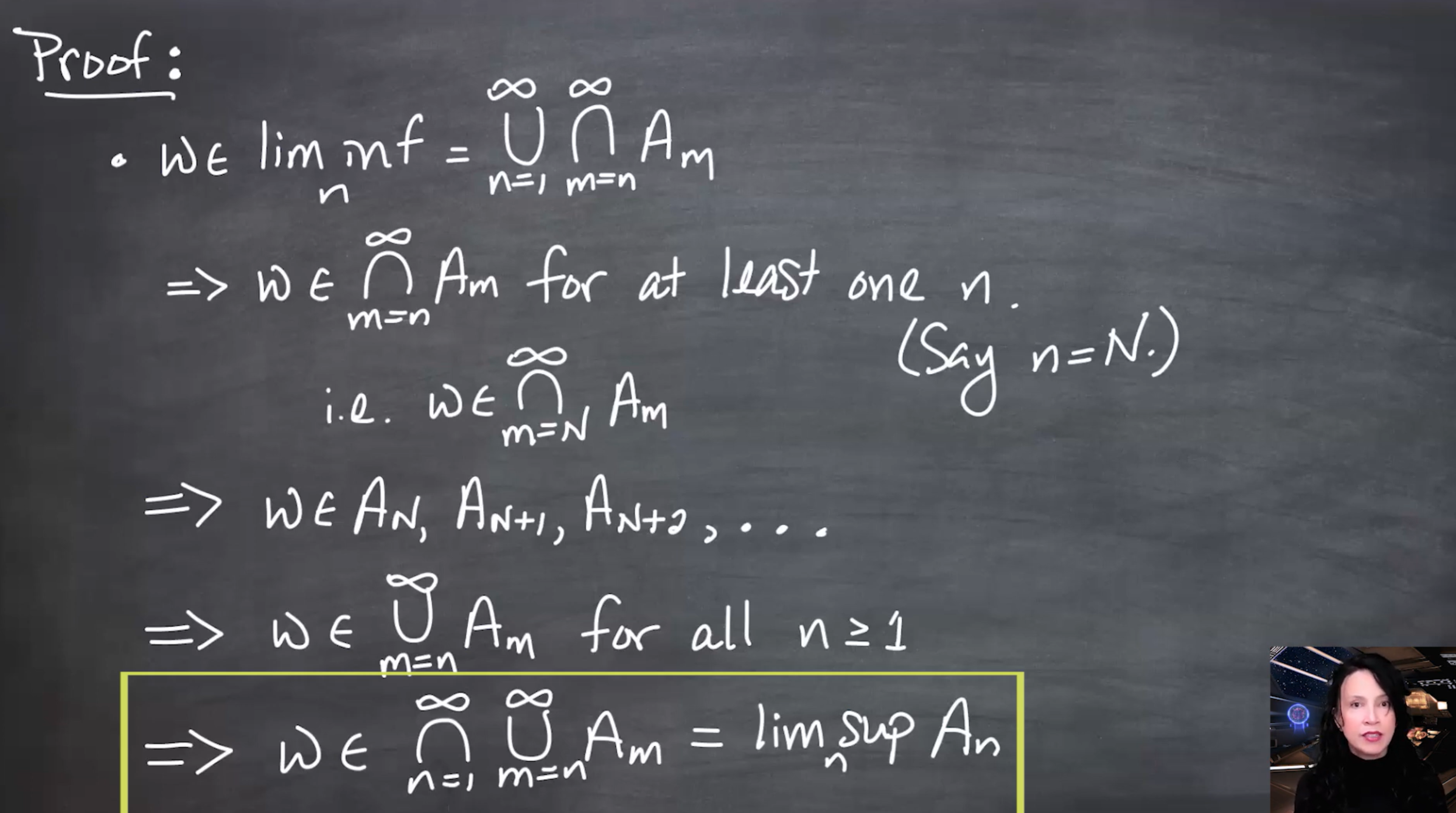
Proof sketch:
Take
\omega\in\liminf A_n = \bigcup_{n=1}^{\infty}\bigcap_{m=n}^{\infty}A_m.
Then for some fixed N,
\omega\in\bigcap_{m=N}^{\infty}A_m.
So \omega\in A_m for every m\geq N. Therefore, for every n, \omega belongs to the tail union
\bigcup_{m=n}^{\infty}A_m.
Hence
\omega\in \bigcap_{n=1}^{\infty} \bigcup_{m=n}^{\infty}A_m = \limsup A_n.
153.9 Definition of the limit of sets
Definition 153.3 (Limit of a sequence of sets) If
\liminf_{n\to\infty}A_n = \limsup_{n\to\infty}A_n,
then the common set is called the limit of the sequence, and we write
\lim_{n\to\infty}A_n = \liminf_{n\to\infty}A_n = \limsup_{n\to\infty}A_n.
If the two sets are not equal, then the sequence of sets does not have a limit.
153.10 Checking the monotone cases
153.10.1 Decreasing case
Suppose
A_1\supseteq A_2\supseteq A_3\supseteq\cdots.
Then
\limsup A_n = \bigcap_{n=1}^{\infty}A_n,
because each tail union is simply its first set:
\bigcup_{m=n}^{\infty}A_m=A_n.
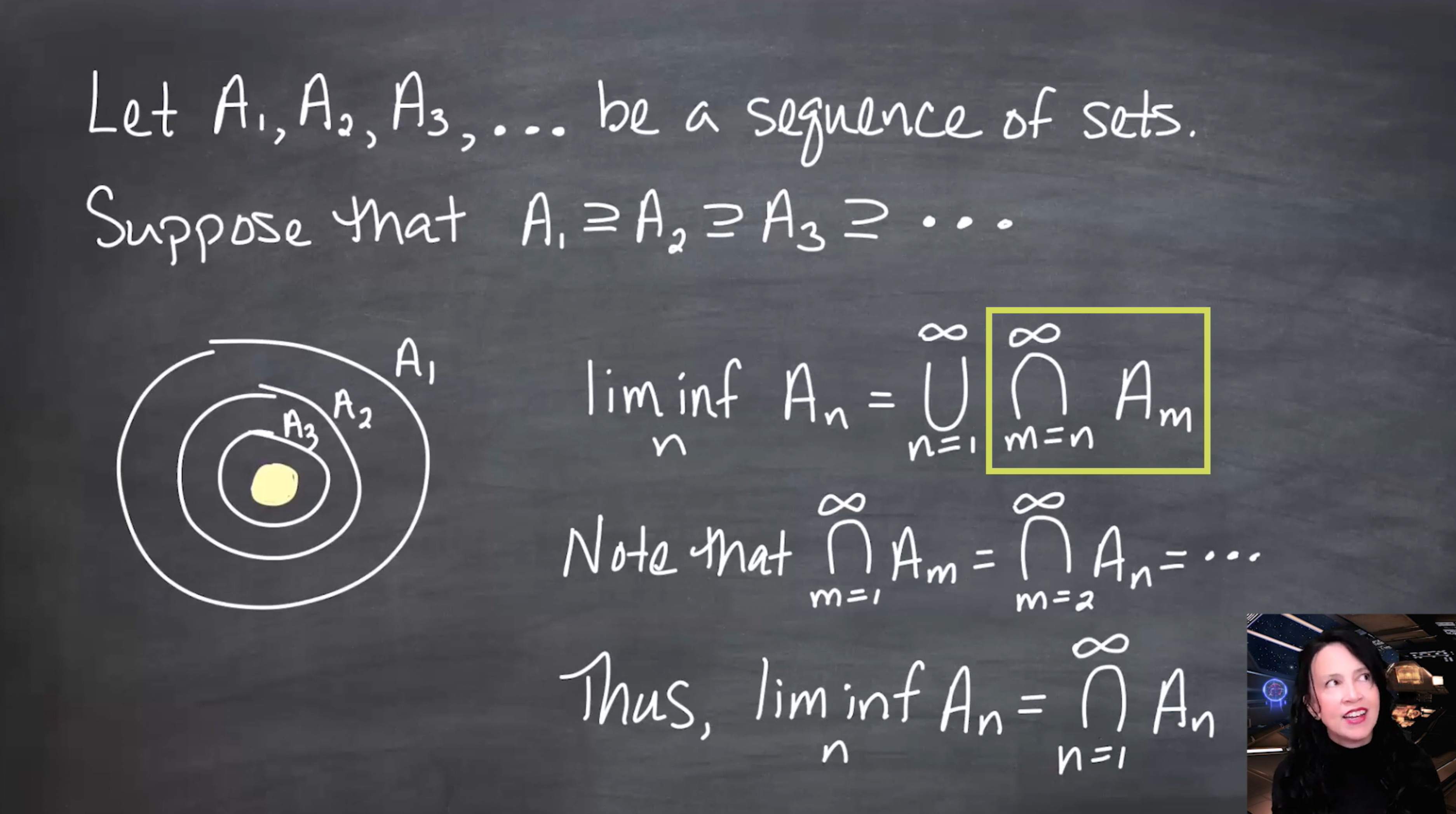
Similarly,
\liminf A_n = \bigcap_{n=1}^{\infty}A_n.
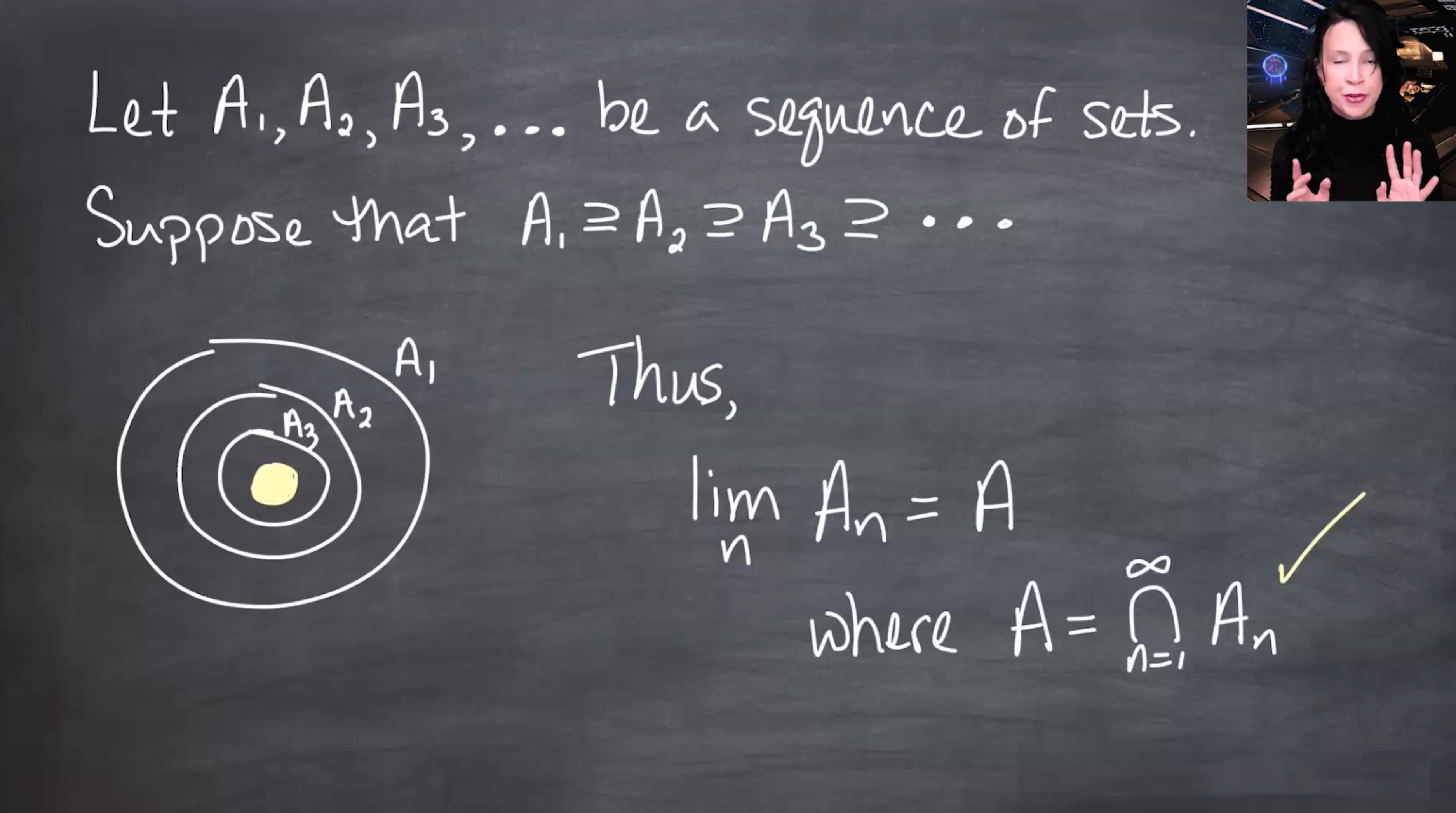
Thus,
A_n\downarrow A \quad\Rightarrow\quad \lim_n A_n=A=\bigcap_{n=1}^{\infty}A_n.
153.10.2 Increasing case
If
A_1\subseteq A_2\subseteq A_3\subseteq\cdots,
then the analogous result is
A_n\uparrow A \quad\Rightarrow\quad \lim_n A_n=A=\bigcup_{n=1}^{\infty}A_n.
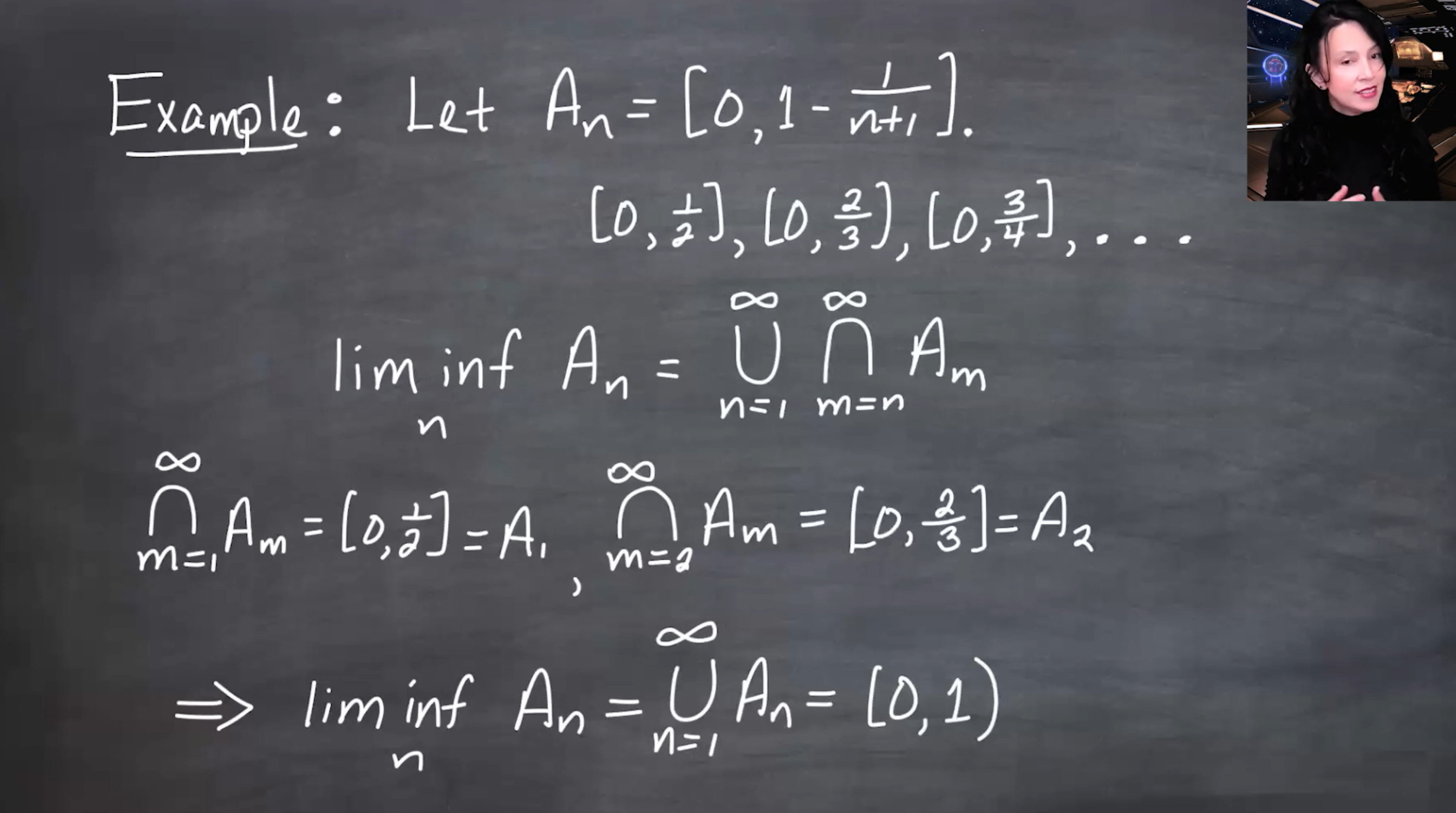
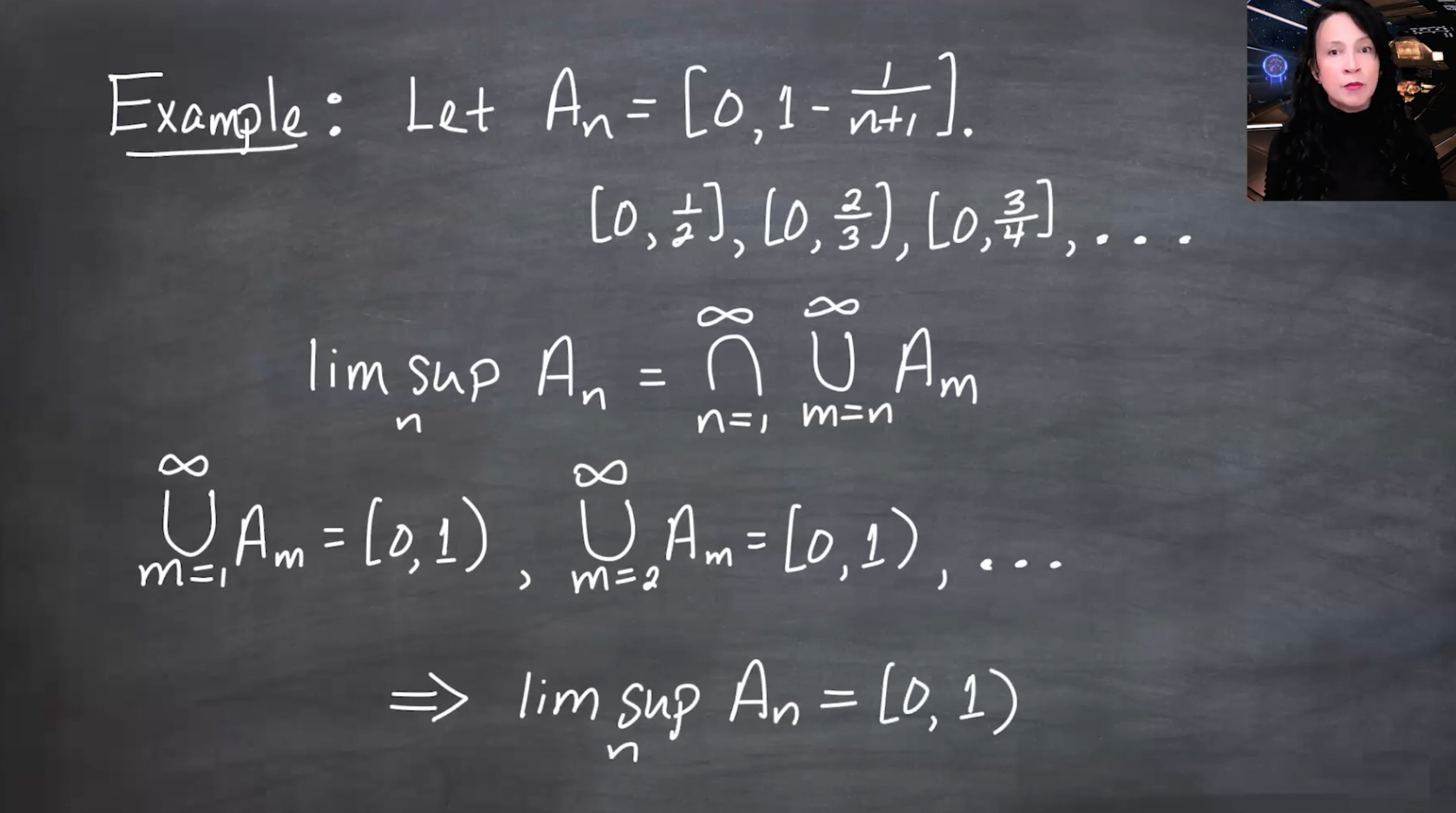
153.11 Revisit the interval example
Recall
A_n=\left[0,1-\frac{1}{n+1}\right].
This is an increasing sequence, so the limit is the union:
\lim_{n\to\infty}A_n = \bigcup_{n=1}^{\infty} \left[0,1-\frac{1}{n+1}\right] = [0,1).
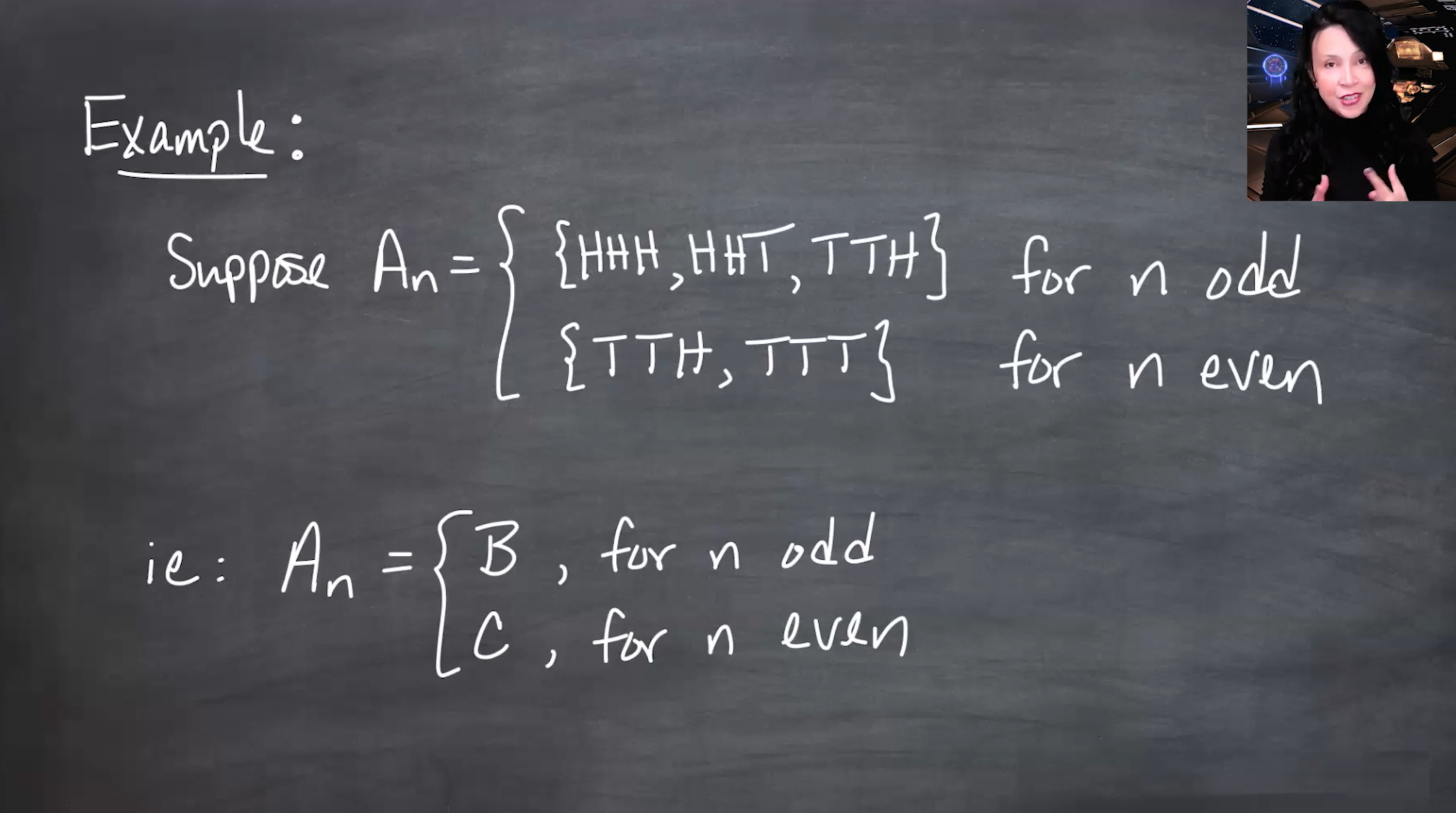
153.12 Alternating sets
Consider a sequence alternating between two sets:
A_n= \begin{cases} B, & n \text{ odd},\\ C, & n \text{ even}. \end{cases}
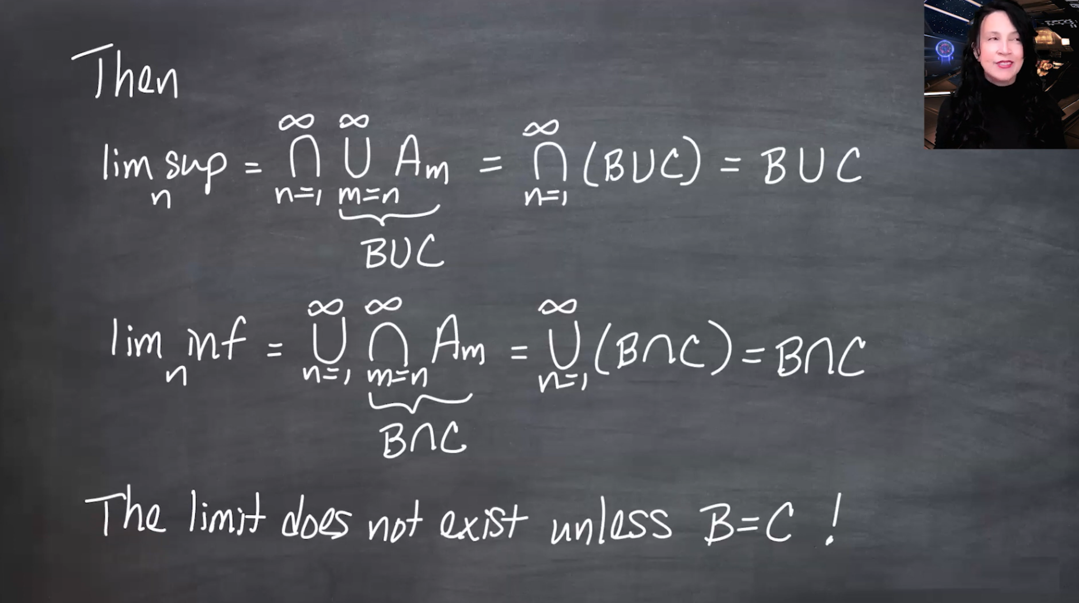
Then every tail union contains both B and C, so
\limsup A_n = B\cup C.
Every tail intersection contains only what is common to both, so
\liminf A_n = B\cap C.
Therefore the limit exists only if
B\cup C = B\cap C,
which happens when B=C.
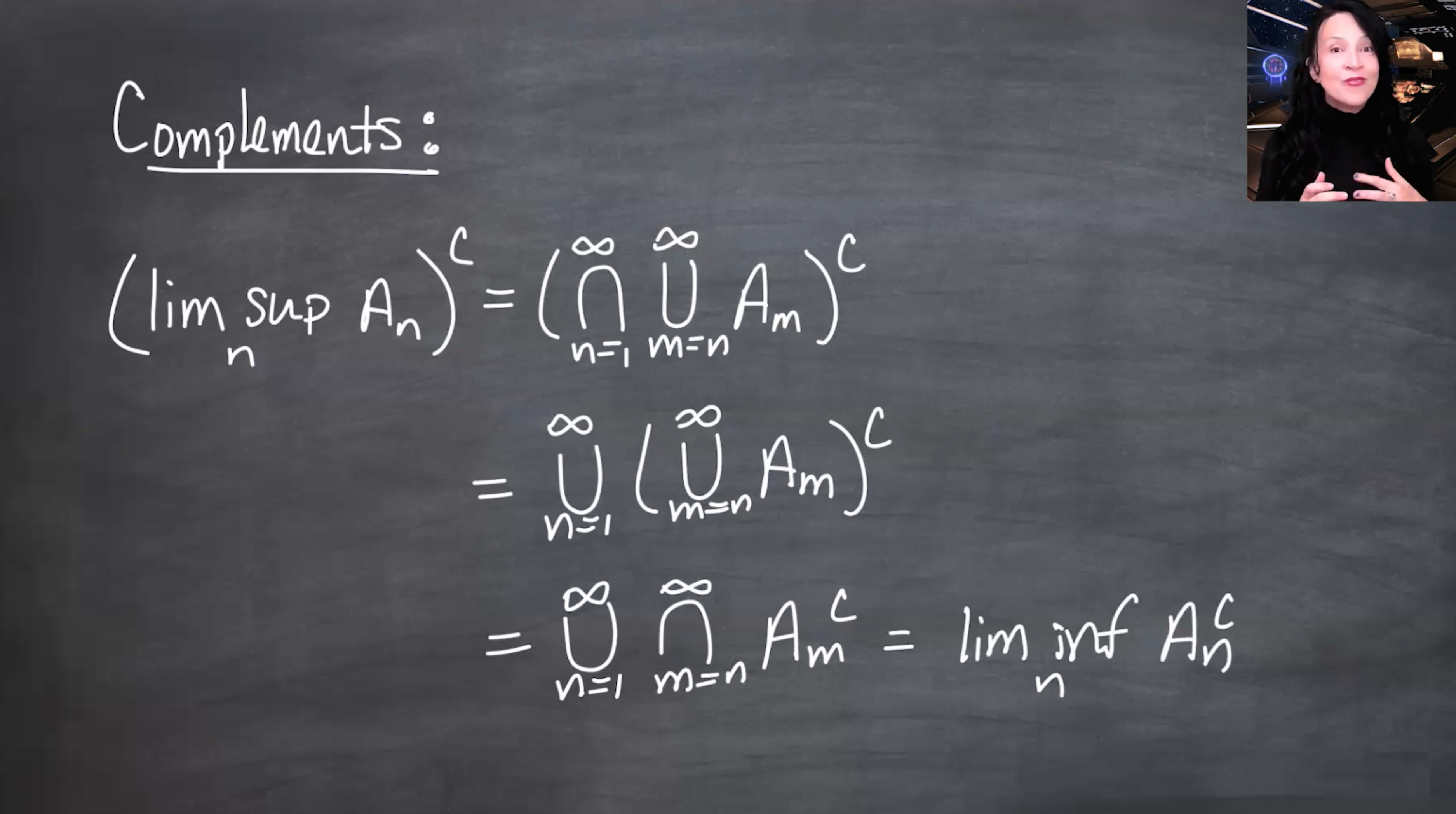
153.13 Complements
The complement of a \limsup is a \liminf of complements:
\left(\limsup_{n\to\infty}A_n\right)^c = \liminf_{n\to\infty}A_n^c.
Using the definition,
\left( \bigcap_{n=1}^{\infty} \bigcup_{m=n}^{\infty}A_m \right)^c = \bigcup_{n=1}^{\infty} \bigcap_{m=n}^{\infty}A_m^c.
This is just De Morgan’s law applied to countable intersections and unions.
Likewise,
\left(\liminf_{n\to\infty}A_n\right)^c = \limsup_{n\to\infty}A_n^c.
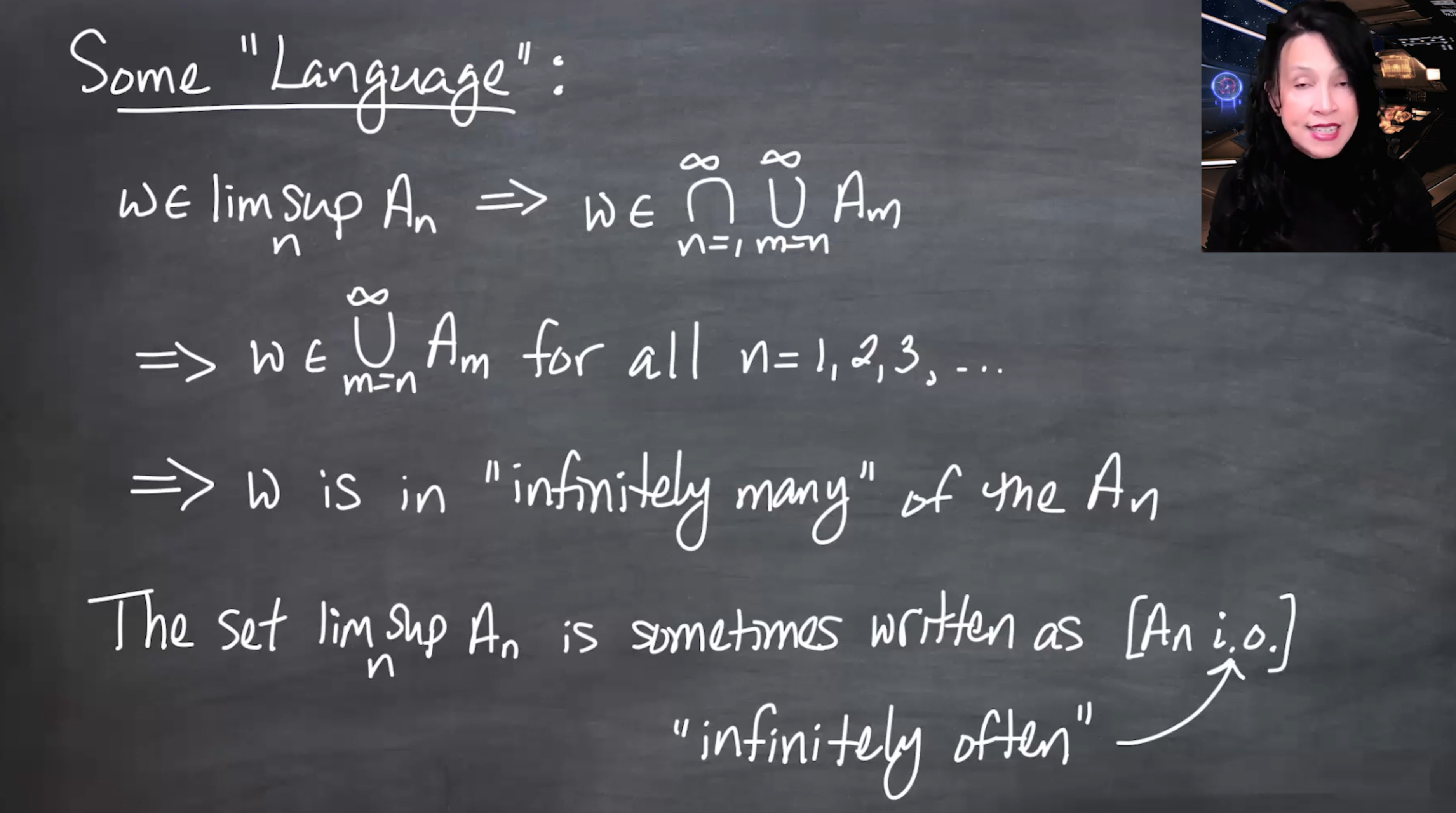
153.14 Event language
The \limsup has a useful event interpretation.
A point \omega is in
\limsup A_n = \bigcap_{n=1}^{\infty}\bigcup_{m=n}^{\infty}A_m
exactly when, no matter how far out in the sequence we go, \omega appears in some later A_m.
So \omega is in infinitely many of the A_n.
This is often written
\limsup A_n = [A_n\ \text{i.o.}],
where i.o. means infinitely often.
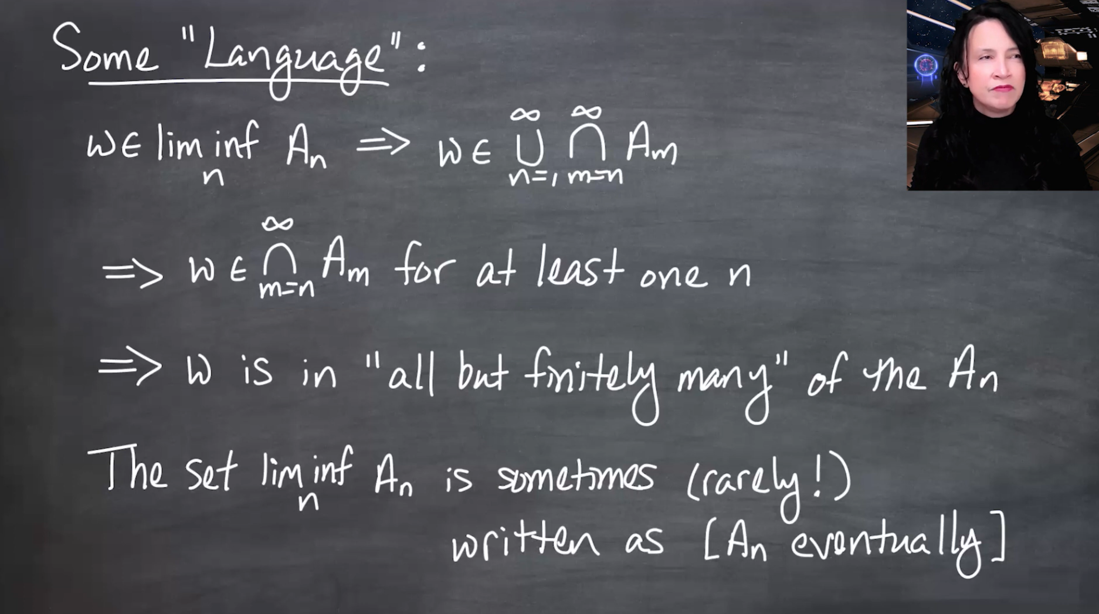
The \liminf means eventual membership:
\liminf A_n = \bigcup_{n=1}^{\infty}\bigcap_{m=n}^{\infty}A_m.
A point \omega is in \liminf A_n when there is some finite time N after which
\omega\in A_m \qquad \text{for all } m\geq N.
That is, \omega belongs to all but finitely many of the A_n.
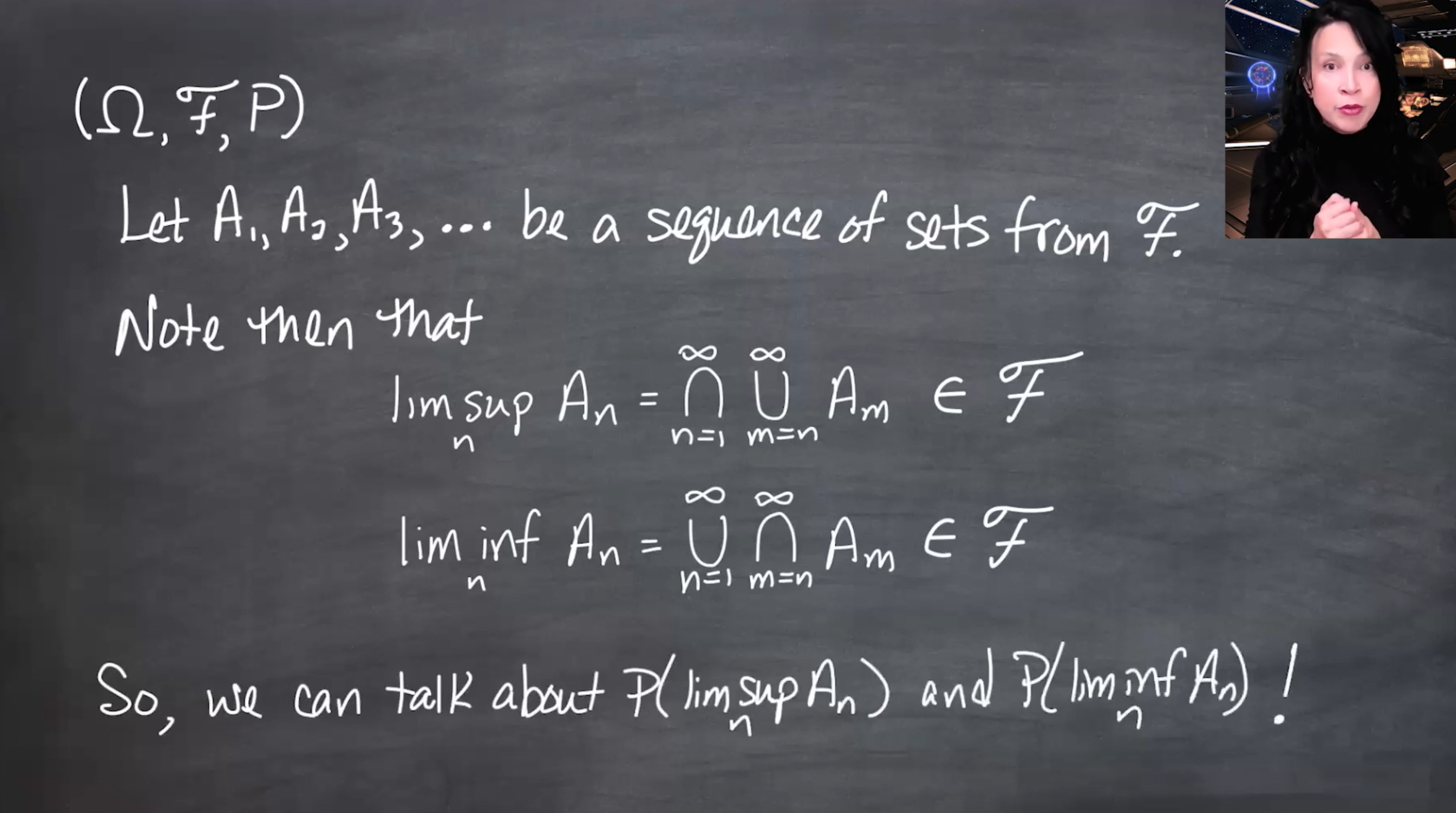
153.15 Measurability of set limits
Suppose (\Omega,\mathcal{F},P) is a probability space and
A_n\in\mathcal{F} \qquad \text{for all } n.
Because \mathcal{F} is a \sigma-field, it is closed under countable unions and intersections. Therefore,
\limsup A_n = \bigcap_{n=1}^{\infty} \bigcup_{m=n}^{\infty}A_m \in\mathcal{F},
and
\liminf A_n = \bigcup_{n=1}^{\infty} \bigcap_{m=n}^{\infty}A_m \in\mathcal{F}.
So it makes sense to discuss
P(\limsup A_n), \qquad P(\liminf A_n).
If the limit exists, then
\lim_n A_n\in\mathcal{F},
so
P\left(\lim_{n\to\infty}A_n\right)
is also well-defined.
153.16 Preview: continuity of probabilities
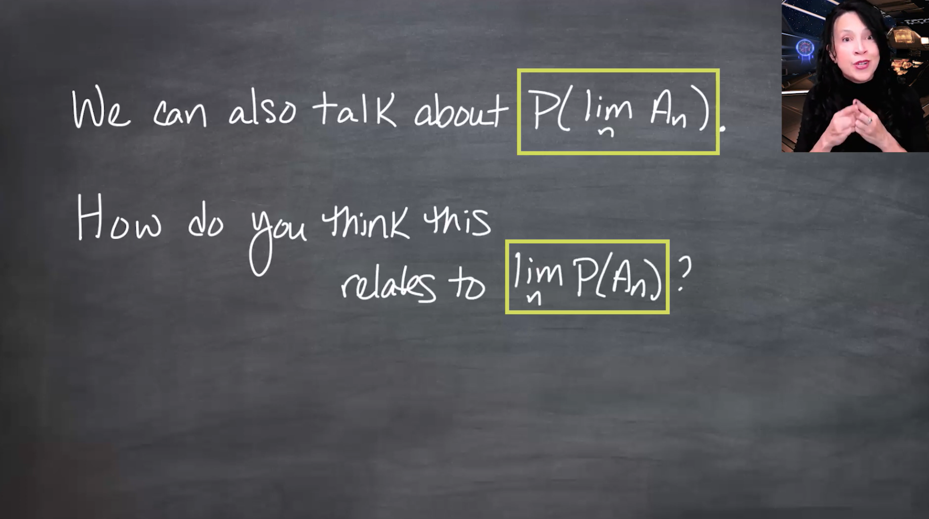
The final question is whether probability commutes with limits of sets.
Compare
P\left(\lim_{n\to\infty}A_n\right)
with
\lim_{n\to\infty}P(A_n).
These are different-looking operations:
- first take a set limit, then measure it;
- first measure each set, then take a numerical limit.
The next lesson studies when these agree. This is called continuity of probabilities.
153.17 Takeaway
The key definitions are:
\limsup_{n\to\infty}A_n = \bigcap_{n=1}^{\infty}\bigcup_{m=n}^{\infty}A_m,
\liminf_{n\to\infty}A_n = \bigcup_{n=1}^{\infty}\bigcap_{m=n}^{\infty}A_m.
The interpretation is:
\limsup A_n = \{\omega:\omega\in A_n \text{ infinitely often}\},
\liminf A_n = \{\omega:\omega\in A_n \text{ eventually}\}.
The limit exists when these two sets are equal.