134.1 Overview of vector random (stochastic) processes
- A stochastic process is a family of random vectors indexed by a parameter set (“time” in our case).
- For example, we might refer to a random process X_k for generic k.
- Value of random process at any specific time k = m is a random variable X_m.
- Usually assume stationarity.
- The statistics (i.e., PDF) of the random variable are time-shift invariant.
- Therefore, \mathbb{E}[X_k] = \bar{x} for all k and \mathbb{E}[X_{k_1} X_{k_2}^T] = R_X(k_1-k_2).
134.2 Properties and important points
Autocorrelation:
R_X(k_1, k_2) = \mathbb{E}[X_{k_1} X_{k_2}^T].
If stationary,
R_X(\tau) = \mathbb{E}[X_k X_{k+\tau}^T].
- Provides a measure of correlation between elements of the process having time displacement \tau.
- R_X(0) = \sigma_X^2 for zero-mean X.
- R_X(0) is always the maximum value of R_X(\tau).
Autocovariance:
C_X(k_1, k_2) = \mathbb{E}\left[(X_{k_1} - \mathbb{E}[X_{k_1}])(X_{k_2} - \mathbb{E}[X_{k_2}])^T\right].
If stationary,
C_X(\tau) = \mathbb{E}\left[(X_k - \bar{x})(X_{k+\tau} - \bar{x})^T\right].
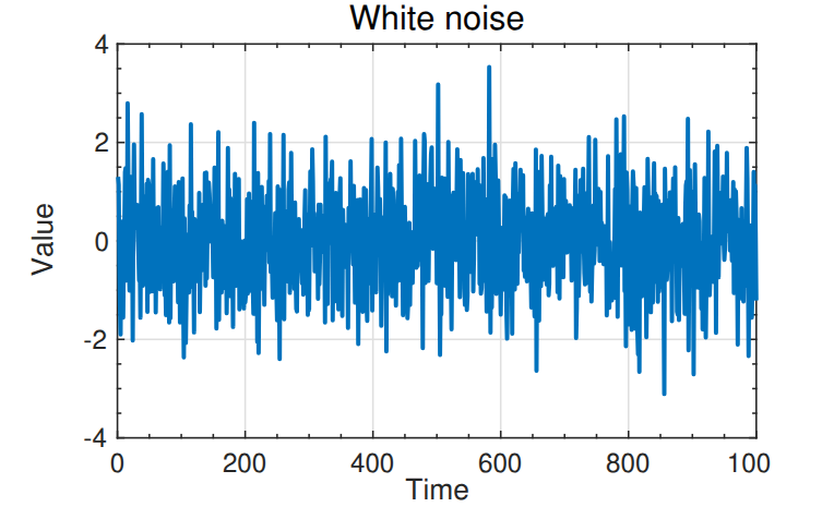
134.3 White noise
- White noise: Some processes have a unique autocorrelation:
Zero mean.
R_X(\tau) = \mathbb{E}[X_k X_{k+\tau}^T] = S_X\,\delta(\tau)
where \delta(\tau) is the Dirac delta, and
\delta(\tau) = 0 \quad \forall\; \tau \neq 0.
- Therefore, the process is uncorrelated in time.
- Clearly an abstraction, but proves to be a very useful one.
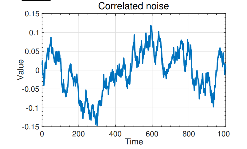
134.4 Shaping filters: Idea
- Will assume noise inputs to dynamic systems are white.
- Limiting assumption, but one that can be easily fixed.
- Can use second linear system to “shape” the noise as desired.
- Limiting assumption, but one that can be easily fixed.
- Can drive our linear system with noise that has desired characteristics by introducing shaping filter H(\cdot) that itself is driven by white noise.
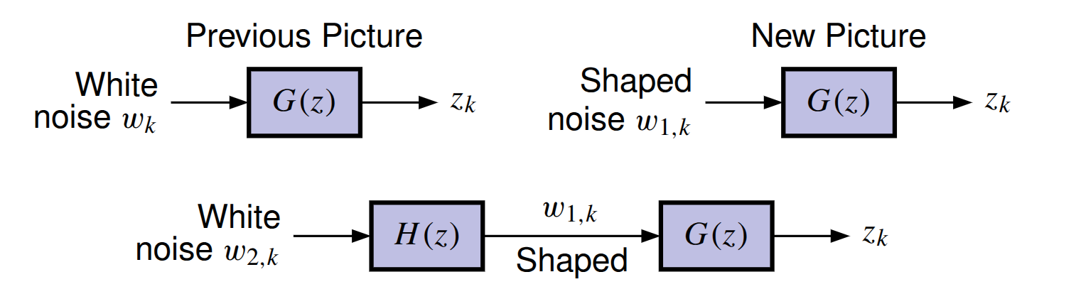
134.5 Shaping filters: Model
- Combined system GH(\cdot) looks exactly the same as before, but G(\cdot) is not driven by pure white noise any more.
- Analysis augments original system model with filter states.
Original system has:
x_{k+1} = A x_k + B_w w_{1,k}
z_k = C x_k.
Shaping filter with white input and desired output statistics has:
x_{s,k+1} = A_s x_{s,k} + B_s w_{2,k}
w_{1,k} = C_s x_{s,k}.
Combine into larger-order augmented system driven by white noise:
\begin{bmatrix} x_{k+1} \\ x_{s,k+1} \end{bmatrix} = \begin{bmatrix} A & B_w C_s \\ 0 & A_s \end{bmatrix} \begin{bmatrix} x_k \\ x_{s,k} \end{bmatrix} + \begin{bmatrix} 0 \\ B_s \end{bmatrix} w_{2,k}
z_k = \begin{bmatrix} C & 0 \end{bmatrix} \begin{bmatrix} x_k \\ x_{s,k} \end{bmatrix}.
134.6 Gaussian processes
- We will work with Gaussian noises to a large extent.
- Uniquely defined by the first- and second central moments of the statistics.
- Gaussian assumption not essential.
- Our filters will always track only the first two moments.
Notation: Until now, we have always used capital letters for random variables.
- The state of a system driven by a random process is a random variable, so we could call it X_k.
- It is more common to retain standard notation x_k and understand from the context that we are discussing a random variable.
134.7 Summary
- Random process is a family of random variables indexed by time.
- Will assume our random processes are stationary.
- Autocorrelation and autocovariance measure self-predictability of a signal at different time offsets.
- White noise is zero mean signal, completely uncorrelated with self (“completely random”).
- An abstraction, but a very useful one.
- If noises in a system of interest are not white, we can model them as filtered white noise to imitate the same general characteristics.
- From now on, unless stated otherwise, all noise signals will be white and Gaussian.