67 The EM algorithm for Mixture models - M2L3

TODO

In the EM algorithm generate animation from the outputs of the algorithm steps + prior & posterior
Add example for carb data

The Expectation-Maximization (EM) algorithm is a broadly applicable statistical technique for maximizing complex likelihoods and handling the incomplete data problem. At each iteration step of the algorithm, two steps are performed:

E-Step consisting of projecting an appropriate functional containing the augmented data on the space of the original, incomplete data, and M-Step consisting of maximizing the functional.

67.0.1 Motivation

In the course the EM algorithm is motivated by the following argument:

Maximum likelihood estimation (MLE) is the preferred estimator used within the frequentist paradigm to infer the parameters of statistical models. However, attempting to obtain (MLEs) \hat{\omega} and \hat{\theta} by directly maximizing the observed-data likelihood:

\mathcal{L}(\omega,\theta) = \arg \max_{\omega,\theta} \prod_{i=1}^{n} \sum_{k=1}^{K} \omega_k g_k(x_i|\theta_k) \tag{67.1}

isn’t feasible in practice, as it is a non-convex optimization problem.

Using numerical optimization methods, such as the Newton-Raphson algorithm, becomes increasingly more challenging when number of components in the mixture increases, as the likelihood surface becomes more complex with multiple local maxima.

67.1 More Motivation: Fisher’s Example

This extended example is not from the Coursera specialization, rather it is due to a 2002 lecture by Terry Speed of UC at Berkeley by way of a handout for ISyE8843A by Brani Vidakovic titled on the EM Algorithm and Mixtures (accessed 2026-06-11). It has been adapted by me - spelling some things out in greater detail. I find that it helps to provide a bit more about Fisher’s Frame of mind as a Statistician who was working on genetics problems in the early 20th century. This is not a toy problem but also not very complicated, and it is a good illustration of the EM algorithm in a setting where the data is incomplete and the likelihood is complex.

Example 67.1 (Fisher’s Example)

67.1.0.1 Glossary of terms

Locus: A specific location on a chromosome where a gene or genetic marker is located.
Allele: A variant form of a gene at a particular locus. Alleles can differ in their DNA sequence and can lead to different traits or phenotypes.
Heterozygote: An individual that has two different alleles at a specific locus, one inherited from each parent.
Gamete: A haploid reproductive cell (sperm or egg) that carries half the genetic information of an organism and fuses with another gamete during fertilization to form a zygote.
Zygote: A diploid cell resulting from the fusion of two haploid gametes during fertilization, containing genetic information from both parents.
Phenotype: The observable physical or biochemical characteristics of an organism, determined by its genotype and environmental factors.
Recombination rate: The frequency at which genetic recombination occurs between two loci during meiosis, leading to the exchange of genetic material between homologous chromosomes.
67.2 Double heterozygote: An individual that is heterozygous at two different loci, having two different alleles at each locus.

67.2.0.1 The problem

In modern terminology, one has two linked bi-allelic loci, A and B say, with alleles A and a, and B and b, respectively, where A is dominant over a and B is dominant over b. A double heterozygote AaBb will produce gametes of four types: AB, Ab, aB and ab. Since the loci are linked, the types AB and ab will appear with a frequency different from that of Ab and aB, say 1 − r and r, respectively, in males, and 1 − r′ and r′ respectively in females. Here we suppose that the parental origin of these heterozygotes is from the mating AABB \times aabb, so that r and r′ are the male and female recombination rates between the two loci.

The problem is to estimate r and r′, if possible, from the offspring of selfed double heterozygotes.

Since gametes are produced in the following proportions:

Table 67.1: Gamete proportions

gamete	male proportion	female proportion
AB	(1 − r)/2	(1 − r')/2
Ab	r/2	r'/2
aB	r/2	r'/2
ab	(1 − r)/2	(1 − r')/2

therefore zygotes are produced in the following proportions:

Table 67.2: Zygote proportions

P1	P2	zygote	proportion	phenotype
AB	AB	AABB	(1 − r)(1 − r')/4	A^∗B^∗
AB	Ab	AaBB	(1 − r)r'/4	A^∗B^∗
AB	aB	AABb	(1 − r)r'/4	A^∗B^∗
AB	ab	AaBb	r r'/4	A^∗B^∗
Ab	AB	AAbb	(1 − r)(1 − r')/4	A^∗b^∗
Ab	Ab	Aabb	(1 − r)r'/4	A^∗b^∗
Ab	aB	AaBb	r(1 − r')/4	A^∗b^∗
Ab	ab	AaBb	r r'/4	A^∗b^∗
aB	AB	aaBB	r(1 − r')/4	a^∗B^∗
aB	Ab	AaBb	r r'/4	A^∗B^∗
aB	aB	aaBB	r r'/4	a^∗B^∗
aB	ab	aaBb	r(1 − r')/4	a^∗b^∗
ab	AB	AaBb	r(1 − r')/4	a^∗B^∗
ab	Ab	AaBb	r r'/4	a^∗B^∗
ab	aB	aaBb	r r'/4	a^∗b^∗
ab	ab	aabb	(1 − r)(1 − r')/4	a^∗b^∗

Table 67.3: Phenotype proportions

phenotype	proportion
A^∗B^∗	9/16
A^∗b^∗	3/16
a^∗B^∗	3/16
a^∗b^∗	1/16

The problem here is this:

Although there are 16 distinct offspring genotypes, taking parental origin into account, the dominance relations imply that we only observe 4 distinct phenotypes, which we denote by A^∗B^∗, A^∗b^∗, a^∗B^∗ and a^∗b^∗.

Here A^∗ (respectively B^∗) denotes the dominant, while a^∗ (respectively b^∗) denotes the recessive phenotype determined by the alleles at A (respectively B)

Thus individuals with genotypes AABB, AaBB, AABb or AaBb, which account for 9/16 gametic combinations (check!), all exhibit the phenotype A^∗B^∗, i.e. the dominant alternative in both characters, while those with genotypes AAbb or Aabb (3/16) exhibit the phenotype A^∗b^∗, those with genotypes aaB and aaBb (3/16) exhibit the phenotype a^∗B^∗, and finally the double recessives aabb (1/16) exhibit the phenotype a^∗b^∗.

It is a slightly surprising fact that the probabilities of the four phenotypic classes are definable in terms of the parameter

\psi = (1 − r)(1 − r')

as follows:

p(a^∗b^∗)=\frac{\psi}{4} (easy to see),
p(a^∗B^∗)=p(A^∗b^∗)=\frac{(1 − \psi)}{4}, while
p(A^∗B^∗)=1 - \text{the sum of the preceding} = \frac{(2 + \psi)}{4}.

Now suppose we have a random sample of n offspring from the selfing of our double heterozygote. Thus the 4 phenotypic classes will be represented roughly in proportion to their theoretical probabilities, their joint distribution being multinomial,

Multinomial\left[n; \frac{(2 + \psi)}{4} , \frac{(1 − \psi)}{4} , \frac{(1 − \psi)}{4} , \frac{\psi}{4}\right]. \tag{67.2}

Note that here neither r nor r′ will be separately estimable from these data, but only the product (1 −r)(1 − r′).

Note that since we know that r ≤ 1/2 and r′ ≤ 1/2, it follows that \psi \ge 1/4

How do we estimate \psi?

(Fisher and Balmukand 1928) discuss a variety of methods that were in the literature at the time they wrote, and compare them with maximum likelihood, which is the method of choice in problems like this.

We describe a variant of their approach to illustrate the EM algorithm.

Let y = (125, 18, 20, 34) be a realization of vector y = (y_1, y_2, y_3, y_4) believed to be coming from the multinomial distribution given in (Equation 67.2).

The probability mass function, given the data, is

g(y, \psi) = \frac{n!}{y_1!y_2!y_3!y_4!} \left(\frac{1}{2} + \frac{\psi}{4}\right)^{y_1} \left(\frac{1}{4} - \frac{\psi}{4}\right)^{y_2+y_3} \left(\frac{\psi}{4}\right)^{y_4}

The log likelihood, and omitting an additive term not containing \psi, is:

\log L(\psi) = y_1 \log(2 + \psi) + (y_2 + y_3) \log(1 - \psi) + y_4 \log(\psi)

By differentiating with respect to \psi one gets

\frac{\partial \log L(\psi)}{\partial \psi} = \frac{y_1}{2 + \psi} - \frac{y_2 + y_3}{1 - \psi} + \frac{y_4}{\psi}

re-arranging for psi gives

Let (a=y_1,; b=y_2+y_3,; c=y_4). With common denominator (\psi(2+\psi)(1-\psi)),

\frac{a}{2+\psi}-\frac{b}{1-\psi}+\frac{c}{\psi} =\frac{,a\psi(1-\psi)-b\psi(2+\psi)+c(2+\psi)(1-\psi),}{\psi(2+\psi)(1-\psi)}.

Expanding the numerator and collecting powers of ():

a\psi(1-\psi)-b\psi(2+\psi)+c(2+\psi)(1-\psi) =-(a+b+c)\psi^2+(a-2b-c)\psi+2c.

Substitute back (a,b,c), the quadratic equation is:

\boxed{(y_1+y_2+y_3+y_4)\psi^2+\bigl(-y_1+2y_2+2y_3+y_4\bigr)\psi-2y_4=0}

so the solution is given by the quadratic formula:

\psi = \frac {y_1 - 2y_2 - 2y_3 - y_4 \pm \sqrt{(-y_1 + 2y_2 + 2y_3 + y_4)^2 +8y_4 (y_1 + y_2 + y_3 +y_4)}}{2(y_1 + y_2 + y_3 + y_4)}

So the equation \frac{\partial \log L(\psi)}{\partial \psi} = 0 can be solved by:

#: label: fisher-psi
y <- c(125, 18, 20, 34)
a <- y[1]
b <- y[2] + y[3]
c <- y[4]
psi <- (a - 2*b - c + sqrt((a - 2*b - c)^2 + 8*c*(a+b+c)))/(2*(a+b+c))
psi

[1] 0.6268215

Assume that instead of original value y_1 the counts y_{11} and y_{12}, such that y_{11} + y_{12} = y_1, could be observed, and that their probabilities are 1/2 and \psi/4, respectively.

The “complete data” can be defined as x = (y_{11}, y_{12}, y_2, y_3, y_4). The probability mass function of incomplete data y is

g(y, \psi) = \sum g_c(x, \psi)

where g_c(x, \psi) = c(x) \left(\frac{1}{2}\right)^{y_{11}} \left(\frac{\psi}{4}\right)^{y_{12}} \left(\frac{1}{4} - \frac{\psi}{4}\right)^{y_2+y_3} \left(\frac{\psi}{4}\right)^{y_4}

c(x) is free of \psi, and the summation is taken over all values of x for which y_{11} + y_{12} = y_1.

The “complete” log likelihood is

\log L_c(\psi) = (y_{12} + y_4) \log(\psi) + (y_2 + y_3) \log(1 - \psi) \tag{67.3}

Our goal is to find the conditional expectation of \log _c(\psi) given y, using the starting point for \psi^{(0)},

Q(\psi, \psi^{(0)}) = E_{\psi^{(0)}} \{\log _c(\psi)|y\}

As \log _c is a linear function in y_{11} and y_{12}, the E-Step is done by simply by replacing y_{11} and y_{12} by their conditional expectations, given y.

Considering Y_{11} to be a random variable corresponding to y_{11}, it is easy to see that

Y_{11} \sim \text{Bin}(y_1, \frac{1/2}{1/2 + \psi^{(0)}/4})

Thus, the conditional expectation of Y_{11} given y_1 is

E_{\psi^{(0)}} (Y_{11}|y_1) = y_{12} \frac{1/2}{1/2 + \psi^{(0)}/4} = y_{11}^{(0)}

Of course,

y_{12}^{(0)} = y_1 - y_{11}^{(0)}

This completes the E-Step part.

In the M-Step one chooses \psi^{(1)} so that Q(\psi, \psi^{(0)}) is maximized.

After replacing y_{11} and y_{12} by their conditional expectations

y_{11}^{(0)} and y_{12}^{(0)}

in the Q-function, the maximum is obtained at

\psi^{(1)} = \frac{y_{12}^{(0)} + y_4}{y_{12}^{(0)} + y_2 + y_3 + y_4} = \frac{y_{12}^{(0)} + y_4}{n - y_{11}^{(0)}}

Now, the E- and M-Steps are alternating.

At the iteration k we have

\psi^{(k+1)} = \frac{y_{12}^{(k)} + y_4}{n - y_{11}^{(k)}}

where

y_{11}^{(k)} = \frac{1}{2} \frac{y_1}{1/2 + \psi^{(k)}/4} \qquad y_{12}^{(k)} = y_1 - y_{11}^{(k)}

we can use the following R code to implement the EM algorithm for this problem:

#: label: fisher-em-port
em_example <- function(y1, y2, y3, y4, tol = 1e-6, start = 0.5) {
  n <- y1 + y2 + y3 + y4
  psi_current <- start
  psi_last <- 0
  
  while (abs(psi_last - psi_current) > tol) {
    # E-step
    y11 <- (1/2 * y1) / (1/2 + psi_current / 4)
    y12 <- y1 - y11
    
    # M-step
    psi_new <- (y12 + y4) / (n - y11)
    
    # Update for next iteration
    psi_last <- psi_current
    psi_current <- psi_new
  }
  
  return(psi_current)
}

em_example(125, 18, 20, 34, 1e-6, 0.5)

[1] 0.6268214

I should mention that MLE is more of a frequentist approach, as it provides point estimates of the parameters rather than a distributional view. In contrast, Bayesian methods we will consider later provide a full posterior distribution of the parameters, which is more informative and allows for uncertainty quantification. However in many complex models where dimensionality is high, researchers are more interested in a point estimate and some uncertainty quantification, so things may not look all that different from the MLE approach.

67.3 EM algorithms for general mixtures 🎥

The EM algorithm comes up a lot in NLP and other fields so it is worthwhile to understand it the way we will do so in the course.

It also important that the EM algorithm we use for mixture models is from the 1970s and is not the same as the general EM algorithm. c.f. (Dempster, Laird, and Rubin 1977)

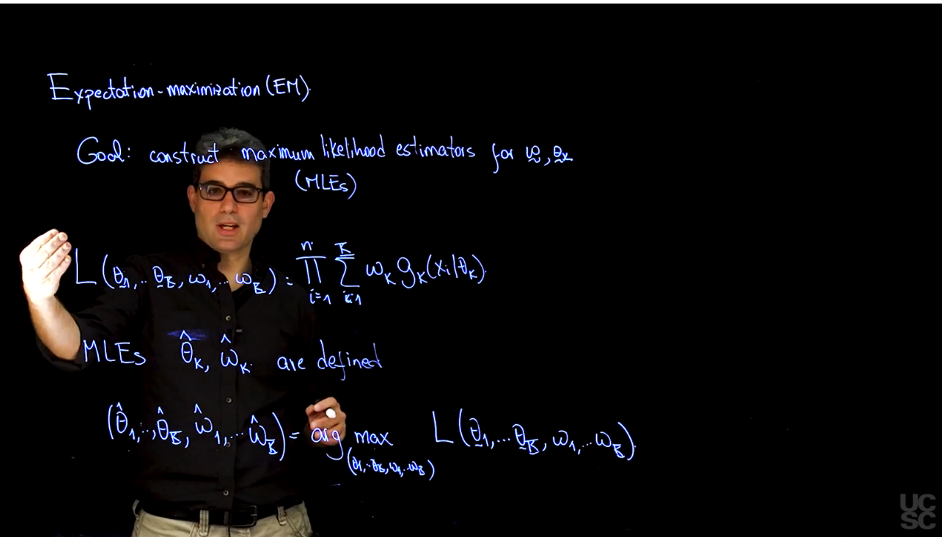
The goal of the EM algorithm is to find the parameters \omega and \theta for which the observed-data likelihood is maximized. We start with the complete-data log-likelihood Q function and then use it to construct maximum likelihood estimators for the parameters we are interested in, these are primarily the weights \omega and the parameters \theta of the distributional components.

we can express the complete-data log-likelihood as:

L(\mathbb{\theta},\mathbb{\omega}) = \prod_{i=1}^{N} \sum_{k=1}^{K} \omega_k g_k(x_i \mid \theta_k) \tag{67.4}

MLE’s \hat{\theta} and \hat{\omega} are defined

(\mathbb{\theta},\mathbb{\omega}) \stackrel{.}{=} \arg \max_{\mathbb{\theta},\mathbb{\omega}} L(\mathbb{\theta},\mathbb{\omega})

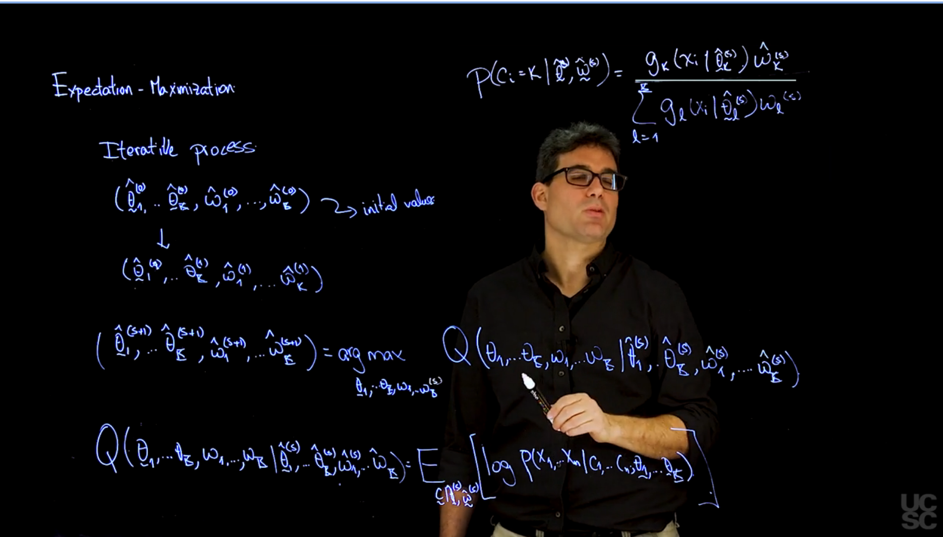
The EM algorithm is iterative and consists of two steps: the E-step and the M-step. The E-step computes the expected value of the complete-data log-likelihood given the observed data and the current parameter estimates, while the M-step maximizes this expected log-likelihood with respect to the parameters. However before we start these steps we need to set initial values for the parameters.

Algorithm 67.1

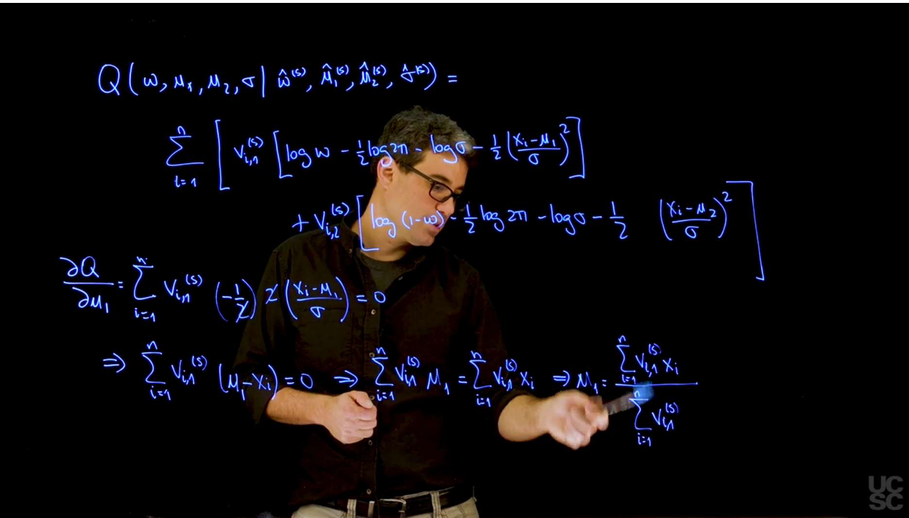
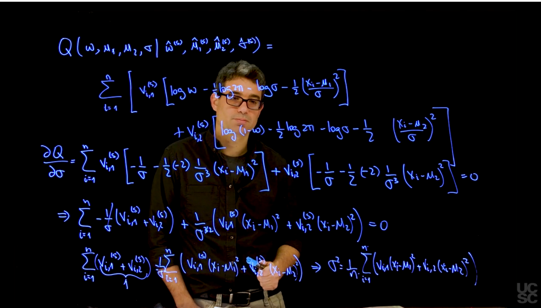
\begin{algorithm} \caption{EM Algorithm for Mixture Models} \begin{algorithmic} \Procedure{EM}{$x, K, \epsilon$} \State Initialize $\omega^{(0)}, \theta^{(0)}$ \State $t \gets 0$ \Repeat \State E-step: Compute $Q(\omega, \theta \mid \omega^{(t)}, \theta^{(t)}, x)$ \State M-step: $(\omega^{(t+1)}, \theta^{(t+1)}) \gets \arg\max_{\omega, \theta} Q(\omega, \theta \mid \omega^{(t)}, \theta^{(t)}, x)$ \State $t \gets t + 1$ \Until{convergence criterion is met (e.g., parameter change or log-likelihood change $< \epsilon$)} \State \Return $\hat{\omega} = \omega^{(t)},\ \hat{\theta} = \theta^{(t)}$ \EndProcedure \end{algorithmic} \end{algorithm}

67.3.1 E step:

Set

Q(\omega,\theta \mid \omega^{(t)}, \theta^{(t)},x) = E_{c \mid \omega^{(t)},\theta^{(t)}, x} \left[ \log \mathbb{P}r(x,c \mid \omega,\theta) \right] \tag{67.5}

Where c is the latent variable indicating the component from which each observation was generated, \omega are the weights, and \theta are the parameters of the Gaussian components (means and standard deviations).

67.3.2 M step:

Set

\hat{\omega}^{(t+1)},\hat{\theta}^{(t+1)} = \arg \max_{\omega,\theta} Q(\omega,\theta \mid \hat{\omega}^{(t)}, \hat{\theta}^{(t)},y) \tag{67.6}

where \hat{\omega}^{(t)} and \hat{\theta}^{(t)} are the current estimates of the parameters, and y is the observed data.

These two steps are repeated until convergence, which is typically defined as the change in the full-data log-likelihood Q function being below a certain threshold.

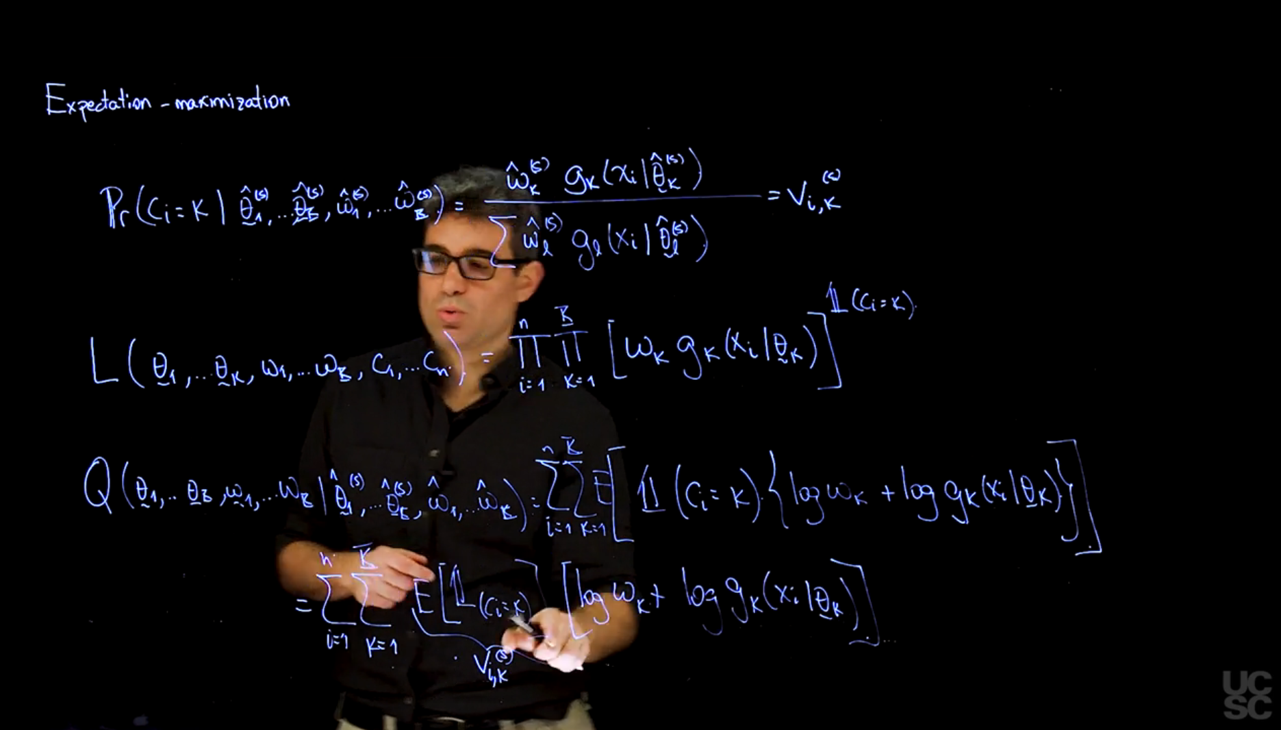
A key point is that if we condition each component independently on the \omega, \theta, x we can write:

\mathbb{P}r(c_i=k \mid \omega, \theta, x_i) = \frac{\omega_k g_k(x_i \mid \theta_k)}{\sum_{j=1}^{K} \omega_j g_j(x_i \mid \theta_j)}= v_{ik}(\omega, \theta)

where the value of v_{ik} is interpreted as the probability that the i^-th observation comes from the k^-th component of the mixture assuming the population parameters \omega and \theta.

67.4 EM for location Mixture of Gaussians 🎥

Figure 67.5: the derivative of Q wrt to w

Figure 67.6: the derivative of Q wrt to mu

Figure 67.7: the derivative of Q wrt to sigma

67.5 EM example 1 🎥

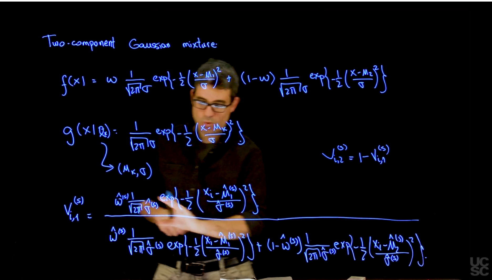
This video covers the code sample given in the listings below. It is a simple implementation of the alg. 67.1 for fitting a 2-component Gaussian location mixture model to simulated data.

This code sample is both cool and awkward.
- It is cool because it provides a step-by-step implementation of the EM algorithm, which is a fundamental concept in statistics and machine learning.
- It is not broken in to functions lacks useful variables naming which would reduce the amounts of comments and cognitive load.
- However it does provide nice visualizations of the alg. 67.1 in action - particularly if run inside of RStudio IDE (as shown in the video).
- would be interesting to make the number of components be drawn from a distribution rather than fixed at 2, then run the EM algorithm for multiple draws and pick the one with the best fit.
- Later on we learn about using BIC to select the number of components in a mixture model, which is a more principled approach than simply fixing the number of components at 2. However it stills seems that the number of components might be a RV even if it’s prior would be centred at the BIC estimate.

67.6 Sample code for EM example 1 🗒️ \mathcal{R}

We start in Listing 67.1 with some house cleaning by clearing the environment and setting the seed for reproducibility.

Listing 67.1: Setup

rm(list=ls())
set.seed(81196)

1: Clear the environment and load required libraries
2: Set the seed for reproducibility of the results.

Since the algorithm will be tested on simulated data, we proceed in Listing 67.2 to generate the synthetic dataset from a mixture of 2 Gaussians.

Listing 67.2: Generate data from a mixture with 2 components

## Ground Truth parameters initialization
KK         = 2
w.true     = 0.6
mu.true    = rep(0, KK)
mu.true[1] = 0
mu.true[2] = 5
sigma.true = 1

n  = 120
cc = sample(1:KK, n, replace=T, prob=c(w.true,1-w.true))
x  = rep(0, n)

for(i in 1:n){ 
  # sample from a distribution with mean selected by component indicator
  # the SD is the same for all components as this is a location mixture
  x[i] = rnorm(1, mu.true[cc[i]], sigma.true)
}

1: Number of components of the mixture
2: Ground Truth (GT) True weights associated with the components
3: Initialize the true means list
4: Ground Truth (GT) True means for each component
5: GT standard deviation of all components
6: Number of synthetic samples to generate
7: Simulate the latent variables for the component indicator function
8: Initialize the data vector x (or load data)

Let us plot the data and the true components before running the EM algorithm.

Listing 67.3: Plotting the synthetic dataset

# Plot the true density
par(mfrow=c(1,1))
xx.true = seq(-8,11,length=200)
yy.true = w.true*dnorm(xx.true, mu.true[1], sigma.true) + 
          (1-w.true)*dnorm(xx.true, mu.true[2], sigma.true) 
plot(xx.true, yy.true, type="l", xlab="x", ylab="True density", lwd=2)
points(x, rep(0,n), col=cc)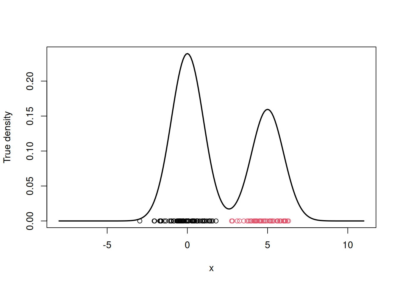

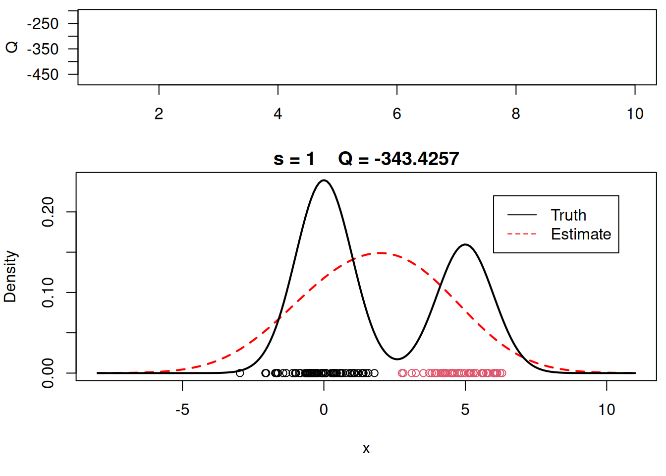
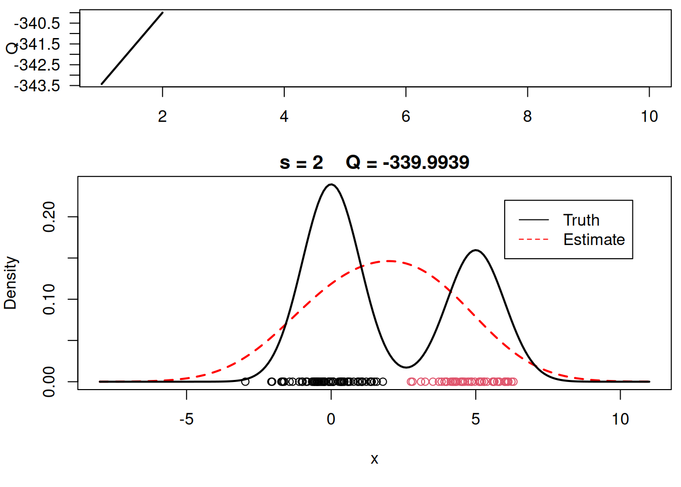
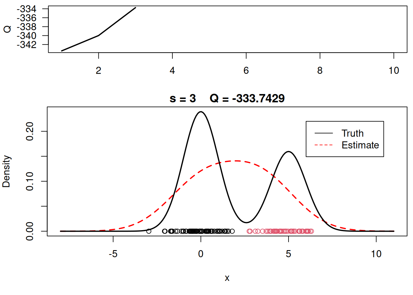
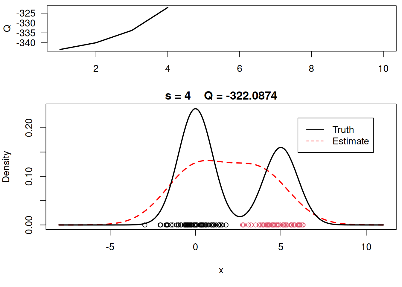
Listing 67.4: Helper function for plotting the EM algorithm for a location mixture of Gaussians

plot_components <- function(  mu, sigma, w, xx, yy.true, x, cc, s, QQ.out){
  # Plot current estimate over data
  layout(matrix(c(1,2),2,1), widths=c(1,1), heights=c(1.3,3))
  par(mar=c(3.1,4.1,0.5,0.5))
  plot(QQ.out[1:s],type="l", xlim=c(1,max(10,s)), las=1, ylab="Q", lwd=2)
  
  par(mar=c(5,4,1.5,0.5))
  xx = seq(-8,11,length=200)
  yy = w*dnorm(xx, mu[1], sigma) + (1-w)*dnorm(xx, mu[2], sigma)
  plot(xx, yy, type="l", ylim=c(0, max(c(yy,yy.true))), main=paste("s =",s,"   Q =", round(QQ.out[s],4)), lwd=2, col="red", lty=2, xlab="x", ylab="Density")
  lines(xx.true, yy.true, lwd=2)
  points(x, rep(0,n), col=cc)
  legend(6,0.22,c("Truth","Estimate"),col=c("black","red"), lty=c(1,2))
}

Now it is time to run the actual EM algorithm - in Listing 67.5 we initialize the parameters of the algorithm.

Listing 67.5: Initialization of the EM algorithm for a location mixture of Gaussians

## Initialize the parameters
w     = 1/2                         # Assign equal weight to each component to start with
mu    = rnorm(KK, mean(x), sd(x))   # Random cluster centers randomly spread over the support of the data
sigma = sd(x)                       # Initial standard deviation

s  = 0
sw = FALSE
QQ = -Inf
QQ.out = NULL
epsilon = 10^(-5)

Mow we can Plot the initial guess for the density

Listing 67.6: Initial parameter estimates of the EM algorithm for a location mixture of Gaussians

xx = seq(-8,11,length=200)
yy = w*dnorm(xx, mu[1], sigma) + (1-w)*dnorm(xx, mu[2], sigma)
plot(xx, yy, type="l", ylim=c(0, max(yy)), xlab="x", ylab="Initial density")
points(x, rep(0,n), col=cc)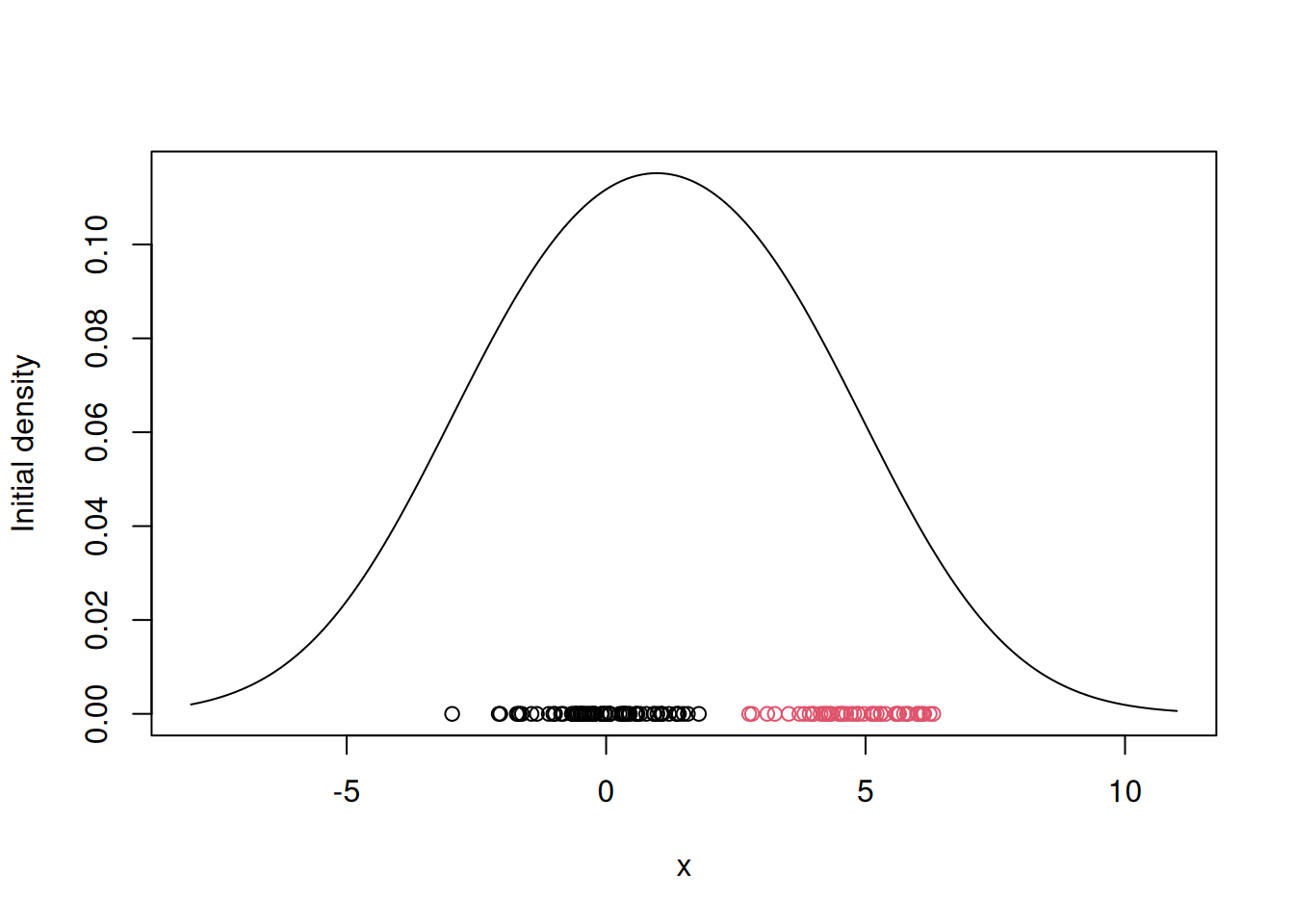

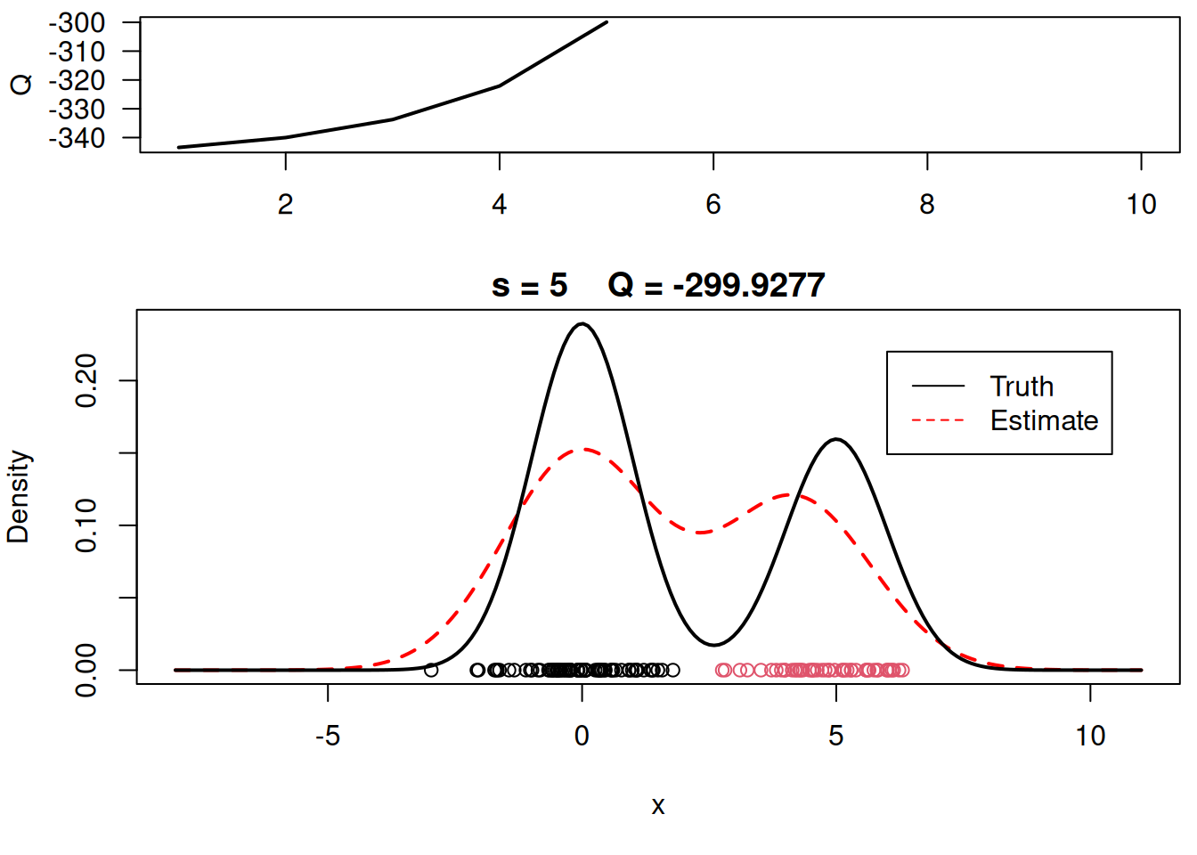
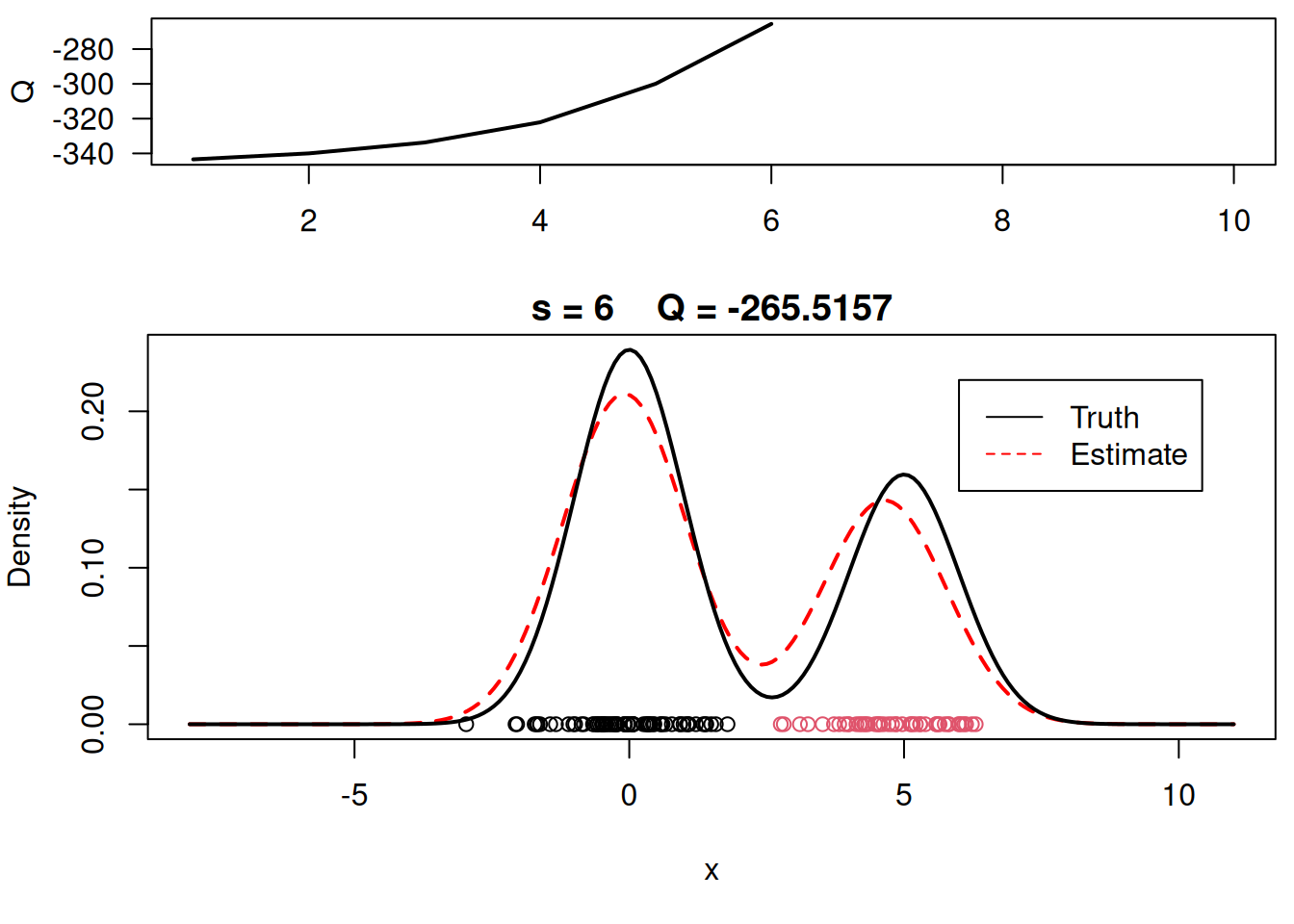
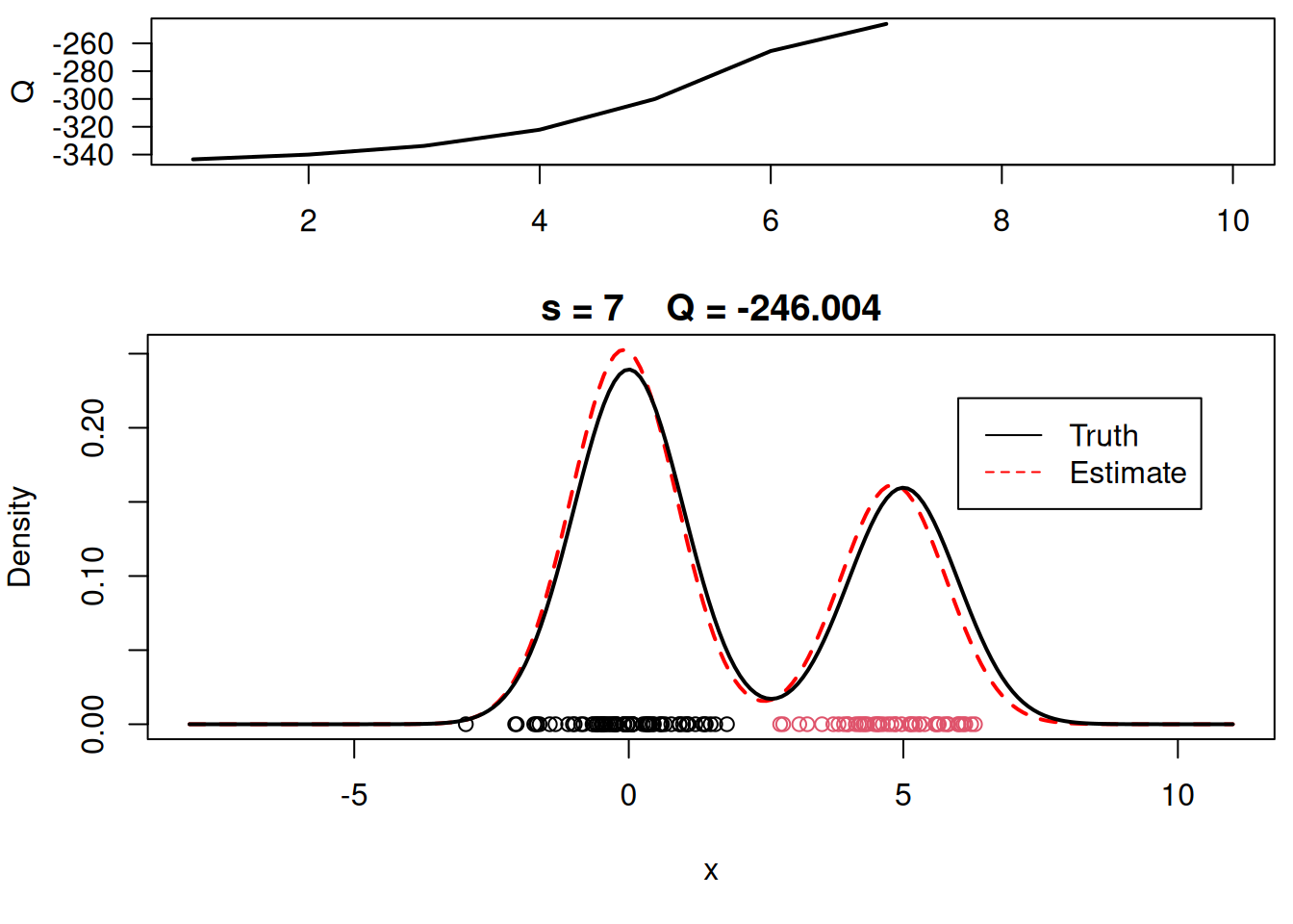
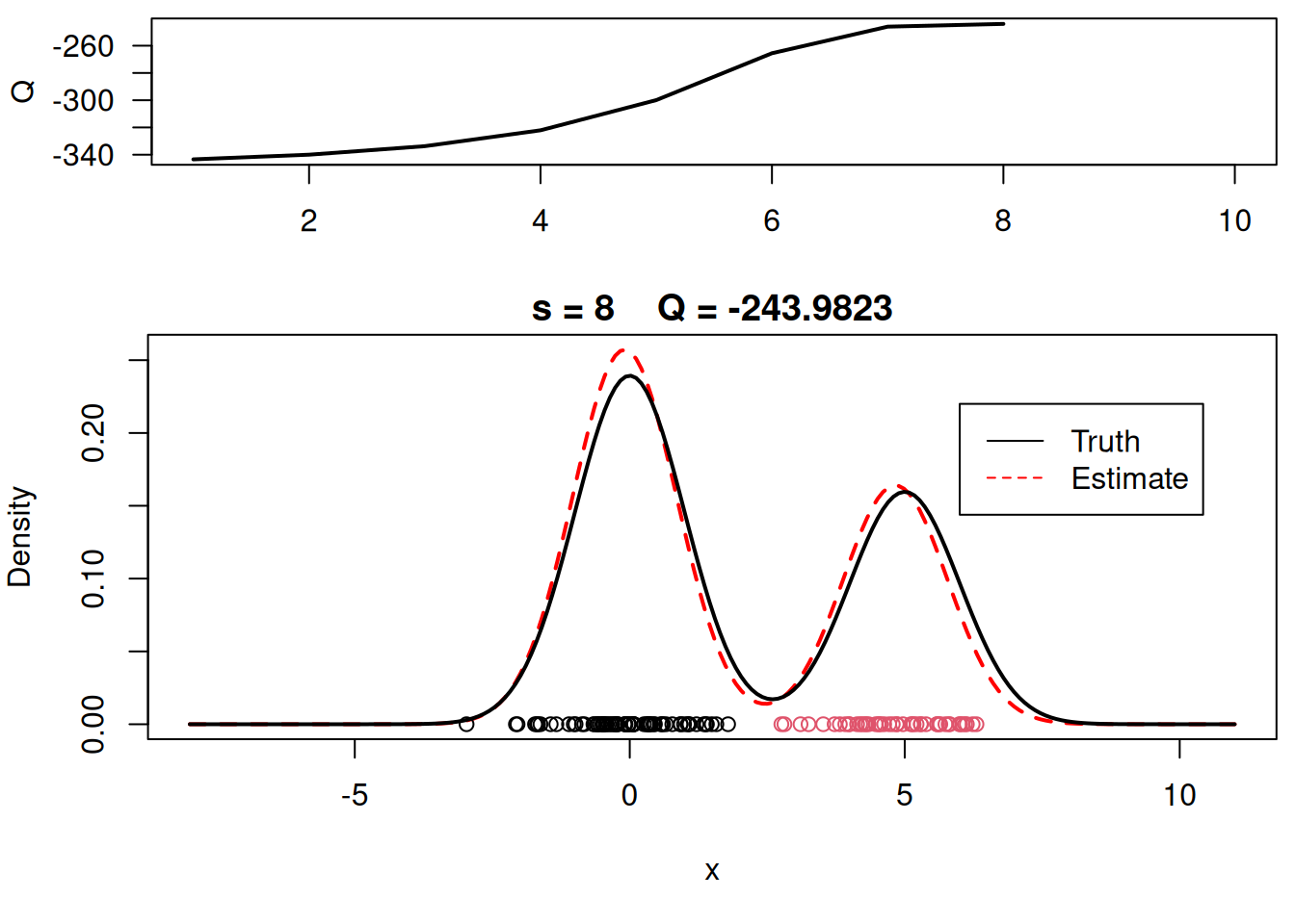
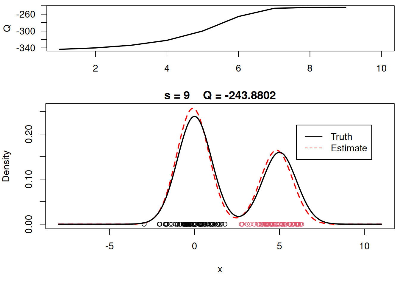
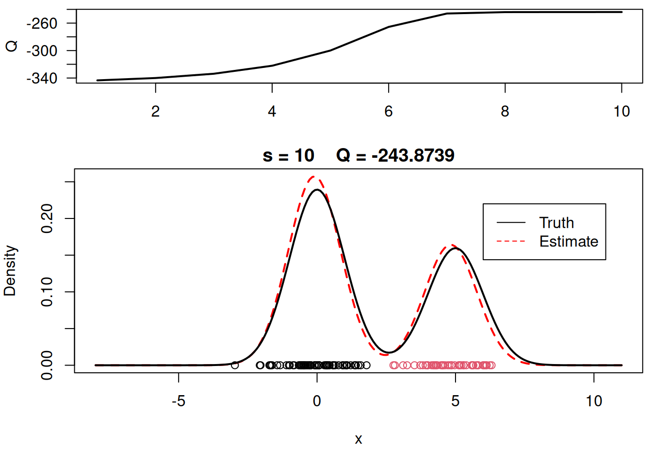
in Listing 67.7 we run the E and M steps until convergence.

Listing 67.7: EM algorithm for a location mixture of Gaussians

## Checking convergence of the algorithm
while(!sw){
  ## E step
  v = array(0, dim=c(n,KK))
  v[,1] = log(w) + dnorm(x, mu[1], sigma, log=TRUE)    # Compute the log of the weights
  v[,2] = log(1-w) + dnorm(x, mu[2], sigma, log=TRUE)  # Compute the log of the weights
  for(i in 1:n){
    v[i,] = exp(v[i,] - max(v[i,]))/sum(exp(v[i,] - max(v[i,])))  #Go from logs to actual weights in a numerically stable manner
  }
  
  ## M step
  # Weights
  w = mean(v[,1])
  mu = rep(0, KK)
  for(k in 1:KK){
    for(i in 1:n){
      mu[k]    = mu[k] + v[i,k]*x[i]
    }
    mu[k] = mu[k]/sum(v[,k])
  }
  # Standard deviations
  sigma = 0
  for(i in 1:n){
    for(k in 1:KK){
      sigma = sigma + v[i,k]*(x[i] - mu[k])^2
    }
  }
  sigma = sqrt(sigma/sum(v))
  
  ##Check convergence
  QQn = 0 # This is the value of the Q function at the new parameter estimates
  for(i in 1:n){
    QQn = QQn + v[i,1]*(log(w)   + dnorm(x[i], mu[1], sigma, log=TRUE)) +
                v[i,2]*(log(1-w) + dnorm(x[i], mu[2], sigma, log=TRUE))
  }
  if(abs(QQn-QQ)/abs(QQn)<epsilon){
    sw=TRUE
  }
  QQ = QQn
  QQ.out = c(QQ.out, QQ)
  s = s + 1
  # print(paste(s, QQn))
  plot_components(mu, sigma, w, xx, yy.true, x, cc, s, QQ.out)

}

Listing 67.8: Final estimate of the EM algorithm

# Plot final estimate over data
layout(matrix(c(1,2),2,1), widths=c(1,1), heights=c(1.3,3))
par(mar=c(3.1,4.1,0.5,0.5))
plot(QQ.out[1:s],type="l", xlim=c(1,max(10,s)), las=1, ylab="Q", lwd=2)

par(mar=c(5,4,1.5,0.5))
xx = seq(-8,11,length=200)
yy = w*dnorm(xx, mu[1], sigma) + (1-w)*dnorm(xx, mu[2], sigma)
plot(xx, yy, type="l", ylim=c(0, max(c(yy,yy.true))), main=paste("s =",s,"   Q =", round(QQ.out[s],4)), lwd=2, col="red", lty=2, xlab="x", ylab="Density")
lines(xx.true, yy.true, lwd=2)
points(x, rep(0,n), col=cc)
legend(6,0.22,c("Truth","Estimate"),col=c("black","red"), lty=c(1,2), bty="n")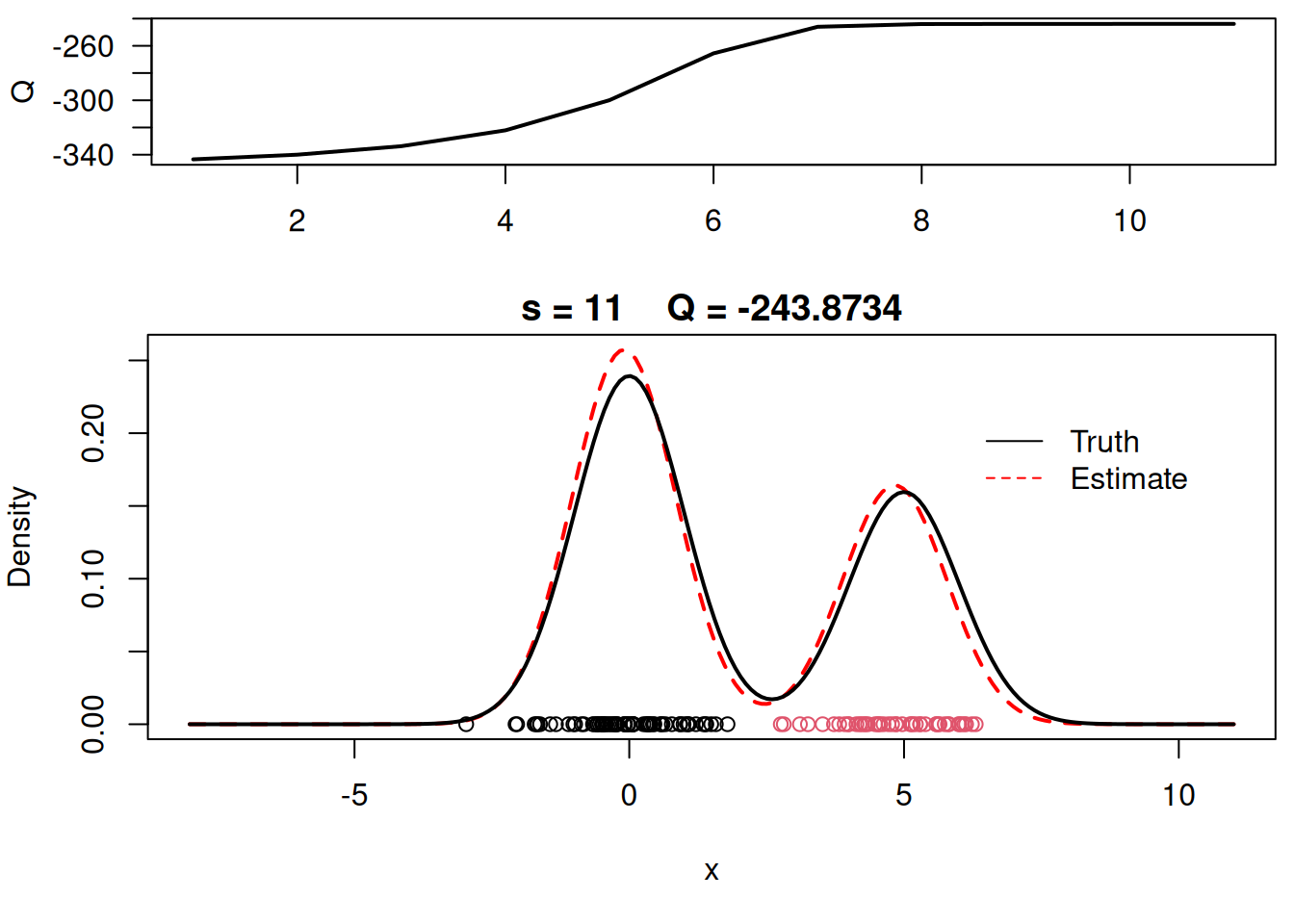

67.7 EM example 2 🎥

This video covers the code sample given in Section 67.8 below. It is a more advanced implementation of the EM algorithm for fitting a mixture of multivariate Gaussian components to simulated data.

67.8 Sample code for multivariate normal EM 🗒️ \mathcal{R}

This variant differs from the code sample above in that it uses the mvtnorm package to generate multivariate normal distributions. It also uses the ellipse package to plot the ellipses around the means of the components.

This is an example of an EM algorithm for fitting a mixtures of K p-variate Gaussian components. The algorithm is tested using simulated data

rm(list=ls())
library(mvtnorm)
library(ellipse)
set.seed(63252)

1: Clear the environment
2: Multivariate normals are not default in R
3: Required for plotting
4: For reproducibility

This code block generates the synthetic data for MVN data using three clusters

## Generate data from a mixture with 3 components
KK      = 3
p       = 2

w.true = c(0.5,0.3,0.2)
mu.true     = array(0, dim=c(KK,p))
mu.true[1,] = c(0,0)
mu.true[2,] = c(5,5)
mu.true[3,] = c(-3,7)

Sigma.true      = array(0, dim=c(KK,p,p))
Sigma.true[1,,] = matrix(c(1,0,0,1),p,p)
Sigma.true[2,,] = matrix(c(2,0.9,0.9,1),p,p)
Sigma.true[3,,] = matrix(c(1,-0.9,-0.9,4),p,p)

n  = 120
cc = sample(1:3, n, replace=T, prob=w.true)
x  = array(0, dim=c(n,p))
for(i in 1:n){
  x[i,] = rmvnorm(1, mu.true[cc[i],], Sigma.true[cc[i],,])
}

1: Number of components of the mixture
2: Number of dimensions of the data
3: True weights associated with the components
4: Initialize the true means list
5: True means for each component
6: Initialize the true variances list
7: True variances for each component
8: Number of synthetic samples to generate
9: Simulate the latent variables for the component indicator function and generate the data
10: Initialize the data matrix x for the sythesized data
11: Sample from a MVN with mean & covariance selected by component indicator

Let us visualize the data and the true components before running the EM algorithm. The ellipses represent the contours of the true Gaussian components at different confidence levels (50%, 82%, and 95%).

par(mfrow=c(1,1))
plot(x[,1], x[,2], col=cc, type="n", xlab=expression(x[1]), ylab=expression(x[2]))
text(x[,1], x[,2], seq(1,n), col=cc, cex=0.6)
for(k in 1:KK){
  lines(ellipse(x=Sigma.true[k,,], centre=mu.true[k,], level=0.50), col="grey", lty=2, lwd=2)
  lines(ellipse(x=Sigma.true[k,,], centre=mu.true[k,], level=0.82), col="grey", lty=2, lwd=2)
  lines(ellipse(x=Sigma.true[k,,], centre=mu.true[k,], level=0.95), col="grey", lty=2, lwd=2)
}
title(main="Data + True Components")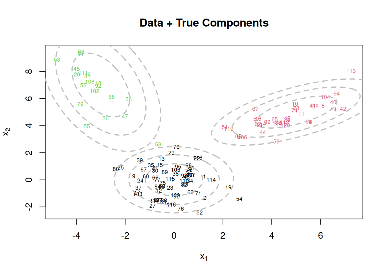

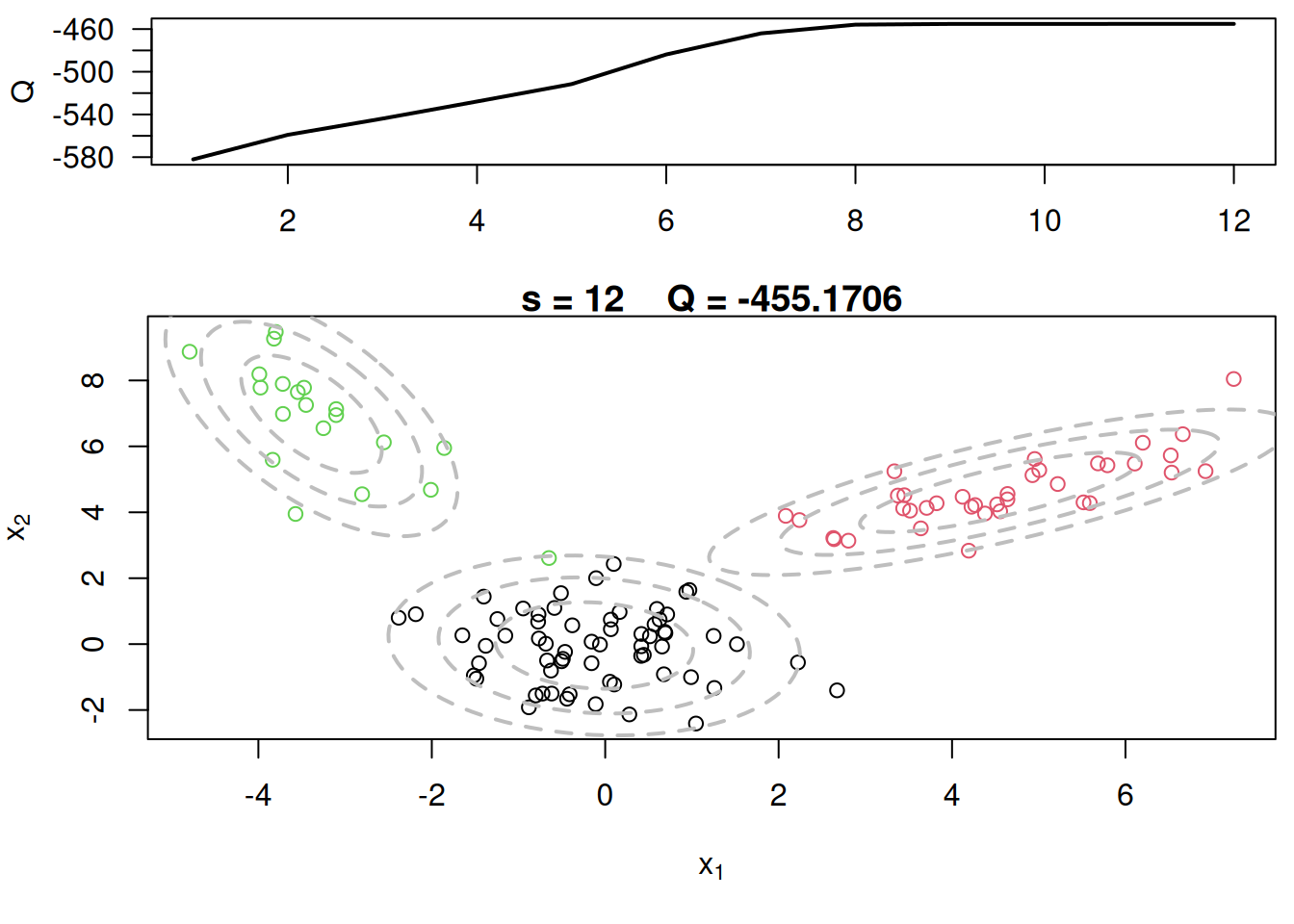
The EM algorithm now fits a mixture of multivariate Gaussian components to the data.

The E-step computes the responsibilities (or weights) for each data point and component, while the M-step updates the parameters (weights, means, and covariances) of the Gaussian components based on these responsibilities. The algorithm iterates until convergence, which is determined by the change in the Q function being below a specified threshold.

plot_components <- function(
  QQ.out, s,
  x, cc,
  KK, Sigma, mu,
  levels = c(0.50, 0.82, 0.95),
  ellipse_col = "grey", ellipse_lty = 2, ellipse_lwd = 2,
  q_ylim = NULL,
  png_dir = NULL, png_prefix = "frame_", png_width = 900, png_height = 700, png_res = 120,

  ...
) {
  
  if (!is.null(png_dir)) {
    dir.create(png_dir, recursive = TRUE, showWarnings = FALSE)
    png_file <- file.path(png_dir, sprintf("%s%03d.png", png_prefix, s))
    grDevices::png(filename = png_file, width = png_width, height = png_height, res = png_res)
    on.exit(grDevices::dev.off(), add = TRUE)
  }

  # Plot current components over data
  layout(matrix(c(1,2),2,1), widths=c(1,1), heights=c(1.3,3))
  par(mar=c(3.1,4.1,0.5,0.5))
  plot(QQ.out[1:s],type="l", xlim=c(1,max(10,s)), las=1, ylab="Q")
  
  par(mar=c(5,4,1,0.5))
  plot(x[,1], x[,2], col=cc, main=paste("s =",s,"   Q =", round(QQ.out[s],4)), 
       xlab=expression(x[1]), ylab=expression(x[2]), lwd=2)
  for(k in 1:KK){
    lines(ellipse(x=Sigma[k,,], centre=mu[k,], level=0.50), col="grey", lty=2, lwd=2)
    lines(ellipse(x=Sigma[k,,], centre=mu[k,], level=0.82), col="grey", lty=2, lwd=2)
    lines(ellipse(x=Sigma[k,,], centre=mu[k,], level=0.95), col="grey", lty=2, lwd=2)
  }
}

1: Set up the layout for the plots
2: Set the margins for the first plot
3: Plot the Q function over iterations
4: Set the margins for the second plot
5: Plot the data points with the current component estimates
6: Draw ellipses for each component at different confidence levels

We can now begin to with the EM algorithm = first we need to initilize the parameters.

w   = rep(1,KK)/KK
mu  = rmvnorm(KK, apply(x,2,mean), var(x))
Sigma      = array(0, dim=c(KK,p,p))
Sigma[1,,] = var(x)/KK
Sigma[2,,] = var(x)/KK
Sigma[3,,] = var(x)/KK

s       = 0
sw      = FALSE
QQ      = -Inf
QQ.out  = NULL
epsilon = 10^(-5)

1: We initially set equal weight to each component
2: We set Random Cluster centers randomly spread over the support of the data
3: We create the covariance matrices with size p \times p for each component.
4: We then initialize them for each component to be the same and equal to the overall covariance of the data divided by the number of components.
5: We initialize the iteration counter,
6: convergence flag,
7: log-likelihood value,
8: vector to store the log-likelihood values over iterations.
9: We set the convergence threshold for the change in log-likelihood between iterations.

Tip

Using a covariance matrix that is the variance of the data scaled down by the number of components is a common initialization strategy that assumes each component starts with a similar spread as the data itself, but scaled down by the number of components to encourage them to capture different parts of the data distribution.
The algorithm will stop when the relative change in log-likelihood is less than this value, indicating that further iterations are unlikely to significantly improve the fit of the model to the data.

par(mfrow=c(1,1))
plot(x[,1], x[,2], col=cc, xlab=expression(x[1]), ylab=expression(x[2]))
for(k in 1:KK){
  lines(ellipse(x=Sigma[k,,], centre=mu[k,], level=0.50), col="grey", lty=2, lwd=2)
  lines(ellipse(x=Sigma[k,,], centre=mu[k,], level=0.82), col="grey", lty=2, lwd=2)
  lines(ellipse(x=Sigma[k,,], centre=mu[k,], level=0.95), col="grey", lty=2, lwd=2)
}
title(main="Initial estimate + Observations")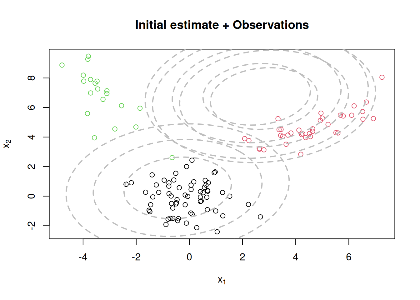

while(!sw){
  ## E step
  v = array(0, dim=c(n,KK))
  for(k in 1:KK){
    v[,k] = log(w[k]) + dmvnorm(x, mu[k,], Sigma[k,,],log=TRUE)  #Compute the log of the weights
  }
  for(i in 1:n){
    v[i,] = exp(v[i,] - max(v[i,]))/sum(exp(v[i,] - max(v[i,])))  #Go from logs to actual weights in a numerically stable manner
  }
  
  ## M step
  w     = apply(v,2,mean)
  mu    = array(0, dim=c(KK, p))
  for(k in 1:KK){
    for(i in 1:n){
      mu[k,]    = mu[k,] + v[i,k]*x[i,]
    }
    mu[k,] = mu[k,]/sum(v[,k])
  }
  Sigma = array(0, dim=c(KK, p, p))
  for(k in 1:KK){
    for(i in 1:n){
      Sigma[k,,] = Sigma[k,,] + v[i,k]*(x[i,] - mu[k,])%*%t(x[i,] - mu[k,])
    }
    Sigma[k,,] = Sigma[k,,]/sum(v[,k])
  }
  
  ## Check convergence
  QQn = 0
  for(i in 1:n){
    for(k in 1:KK){
      QQn = QQn + v[i,k]*(log(w[k]) + dmvnorm(x[i,],mu[k,],Sigma[k,,],log=TRUE))
    }
  }
  if(abs(QQn-QQ)/abs(QQn)<epsilon){
    sw=TRUE
  }
  QQ = QQn
  QQ.out = c(QQ.out, QQ)
  s = s + 1
  #print(paste(s, QQn))
  
  plot_components(QQ.out, s, x, cc, KK, Sigma, mu, c(-200, -100), png_dir = "em_mvn_frames")

}

library(magick)

Linking to ImageMagick 6.9.12.98
Enabled features: fontconfig, freetype, fftw, heic, lcms, pango, raw, webp, x11
Disabled features: cairo, ghostscript, rsvg

Using 4 threads

make_em_gif <- function(
  frames_dir = ".",
  pattern = "frame_*.png",
  out_file = "em.gif",
  duration_sec = 60
) {
  stopifnot(requireNamespace("magick", quietly = TRUE))

  files <- sort(Sys.glob(file.path(frames_dir, pattern)))
  if (length(files) == 0) stop("No frames found. Check frames_dir/pattern.")

  target_fps <- length(files) / duration_sec
  allowed <- c(1, 2, 4, 5, 10, 20, 25, 50, 100)
  fps <- allowed[which.min(abs(allowed - target_fps))]

  img <- magick::image_read(files)
  img <- magick::image_animate(img, fps = fps)
  magick::image_write(img, path = out_file)

  message(sprintf("Wrote %s (%d frames at %d fps ≈ %.1f sec)",
                  out_file, length(files), fps, length(files)/fps))
  invisible(out_file)
}

make_em_gif("em_mvn_frames", out_file = "em.gif", duration_sec = 60)

Wrote em.gif (12 frames at 1 fps ≈ 12.0 sec)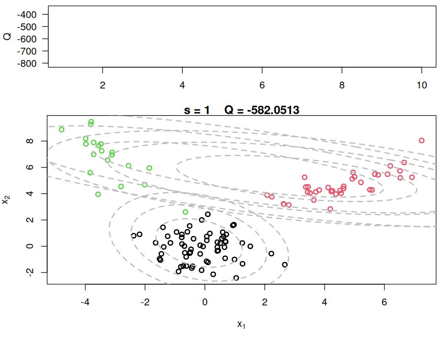

# Plot current components over data
layout(matrix(c(1,2),2,1), widths=c(1,1), heights=c(1.3,3))
par(mar=c(3.1,4.1,0.5,0.5))
plot(QQ.out[1:s],type="l", xlim=c(1,max(10,s)), las=1, ylab="Q", lwd=2)

par(mar=c(5,4,1,0.5))
plot(x[,1], x[,2], col=cc, main=paste("s =",s,"   Q =", round(QQ.out[s],4)), xlab=expression(x[1]), ylab=expression(x[2]))
for(k in 1:KK){
  lines(ellipse(x=Sigma[k,,], centre=mu[k,], level=0.50), col="grey", lty=2, lwd=2)
  lines(ellipse(x=Sigma[k,,], centre=mu[k,], level=0.82), col="grey", lty=2, lwd=2)
  lines(ellipse(x=Sigma[k,,], centre=mu[k,], level=0.95), col="grey", lty=2, lwd=2)
}

67.9 Mixture of Log Gaussians

Prompt

If your data had support on the positive real numbers rather than the whole real line, how could you use the EM algorithm you just learned to instead fit a mixture of log-Gaussian distributions?

Would you need to recode your algorithm?

Response

Updating the algorithm is nontrivial - it requires derivatives for each parameter. Depending on the distribution, we may need to add custom code to update each. We also need to update the distribution if these are changed.

So while the algorithm does not change, the code may change quite a bit.

67.10 Advanced EM algorithms

67.10.1 HW: The EM for ZIP mixtures

Data on the lifetime (in years) of fuses produced by the ACME Corporation is available in the file fuses.csv:

Provide the EM algorithm to fit the mixture model

67 The EM algorithm for Mixture models - M2L3

67.0.1 Motivation

67.1 More Motivation: Fisher’s Example

67.1.0.1 Glossary of terms

67.2 Double heterozygote: An individual that is heterozygous at two different loci, having two different alleles at each locus.

67.2.0.1 The problem

67.3 EM algorithms for general mixtures 🎥

67.3.1 E step:

67.3.2 M step:

67.4 EM for location Mixture of Gaussians 🎥

67.5 EM example 1 🎥

67.6 Sample code for EM example 1 🗒️ \mathcal{R}

67.7 EM example 2 🎥

67.8 Sample code for multivariate normal EM 🗒️ \mathcal{R}

67.9 Mixture of Log Gaussians

Response

67.10 Advanced EM algorithms

67.10.1 HW: The EM for ZIP mixtures

67.10.2 HW+: The EM for Mixture Models