if (!require("pacman")) install.packages("pacman")

Loading required package: pacman

pacman::p_load(faraway)

Installing package into '/home/oren/work/blog/renv/library/R-4.4/x86_64-pc-linux-gnu'
(as 'lib' is unspecified)

also installing the dependencies 'minqa', 'nloptr', 'RcppEigen', 'lme4'


faraway installed

I took this course on Coursera in primarily to get a more solid foundation in time series analysis and forecasting before taking the bayesian time series course. I have some experience with time series analysis from reading a few books and papers, but I wanted to get a more solid foundation in the subject.

Most of the material in this course is introductory and I did not bother with very in depth explanations or notes, often listing just what is covered.

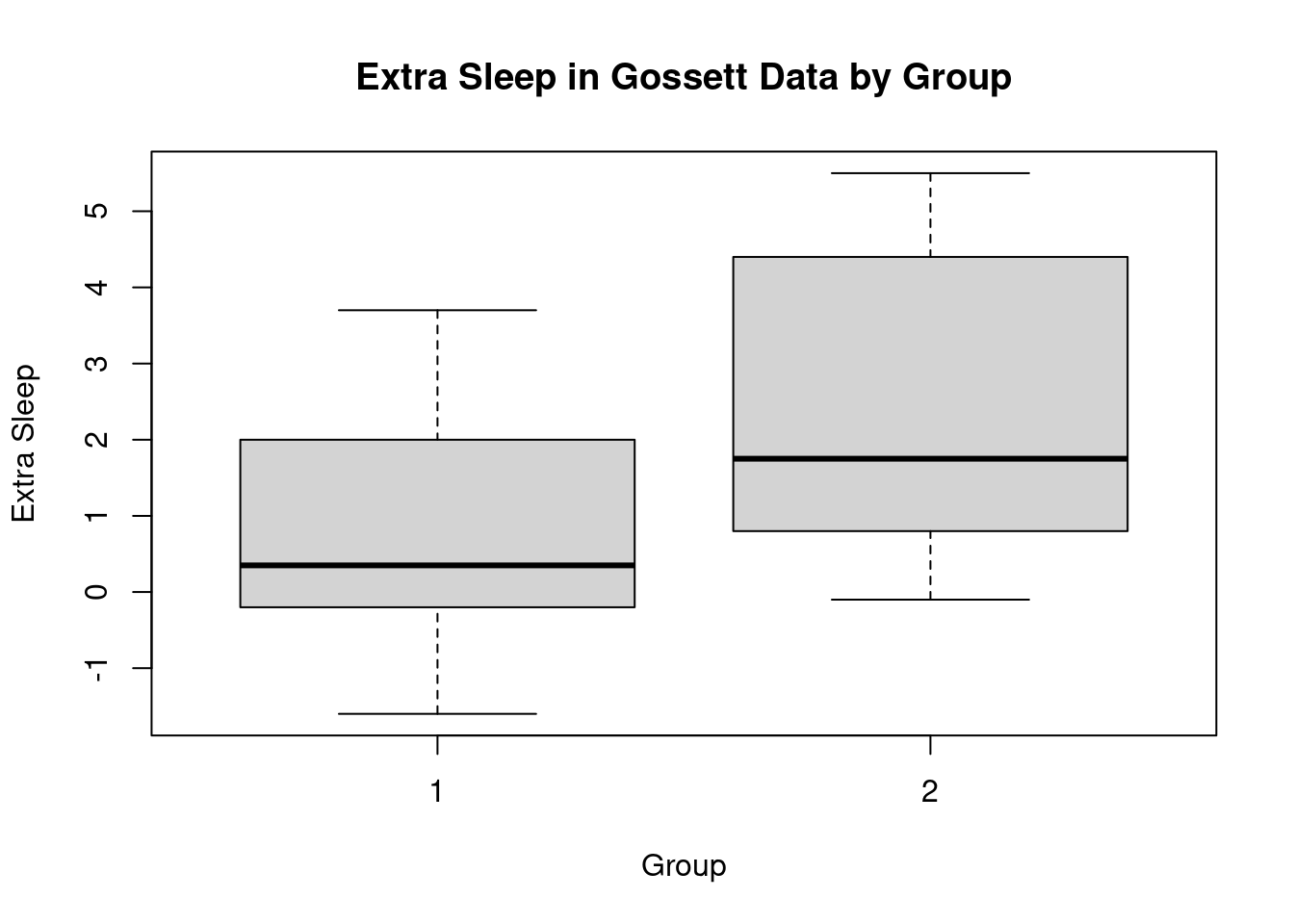
reading for week 1:

Module 1

We begin with the usual pleasantries, and
R software installation
How to load a library
How to load a dataset from a library
Getting some info on the dataset using e.g. help(c02) for the Mauna Loa CO2 dataset.
How to get a five point summary using summary function
How to visualize a dataset with a histogram in R with the hist function
- Customize title, x-label, y-label, color, and breaks
- How to add a density plot to a histogram
How to visualize a bivariate dataset with a scatter plot in R using plot function
- Customize title, x-label, y-label,
- How to add a regression line to a scatter plot with the abline function
How to fit a liner regression model to a dataset in R using lm function
- How we interpret the output of the lm function
- How to get the coefficients of the model using coef function
- Understanding the error term in the regression model
- Talks about some logical assumptions of the linear regression model ¹
  - Normally distributed errors
  - same variance of errors (homoscedasticity)
  - independent errors (no autocorrelation)
- using () around an expression to coerce the output to the console

require(graphics)
summary(co2)

   Min. 1st Qu.  Median    Mean 3rd Qu.    Max. 
  313.2   323.5   335.2   337.1   350.3   366.8

co2lm = lm(co2 ~ time(co2))

# plot data and fit
plot(co2, main='CO2 data', xlab='Time', ylab='CO2')
abline(co2lm, col='red')

co2lm.residuals = residuals(co2lm)

# check the residuals
plot(co2lm.residuals~time(co2), main='Residuals', xlab='Time', ylab='Residuals')

# check the normality of the residuals
qqnorm(residuals(co2lm))
qqline(residuals(co2lm))

library(faraway)
plot(punting$Distance~ punting$Hang); 
abline( lm(punting$Distance~ punting$Hang) )

m=lm(punting$Distance~ punting$Hang) 
qqnorm(resid(m)) 
qqline(resid(m))

using t.test

attach(sleep)
plot(extra~group,data=sleep,main="Extra Sleep in Gossett Data by Group",xlab="Group",ylab="Extra Sleep")

extra_1=extra[group==1]
extra_2=extra[group==2]
t.test(extra_1,extra_2,paired=TRUE,alternative="two.sided")


    Paired t-test

data:  extra_1 and extra_2
t = -4.0621, df = 9, p-value = 0.002833
alternative hypothesis: true mean difference is not equal to 0
95 percent confidence interval:
 -2.4598858 -0.7001142
sample estimates:
mean difference 
          -1.58

the confidence interval does not contain zero, so we can reject the null hypothesis that the means are equal, and conclude that the means are different.

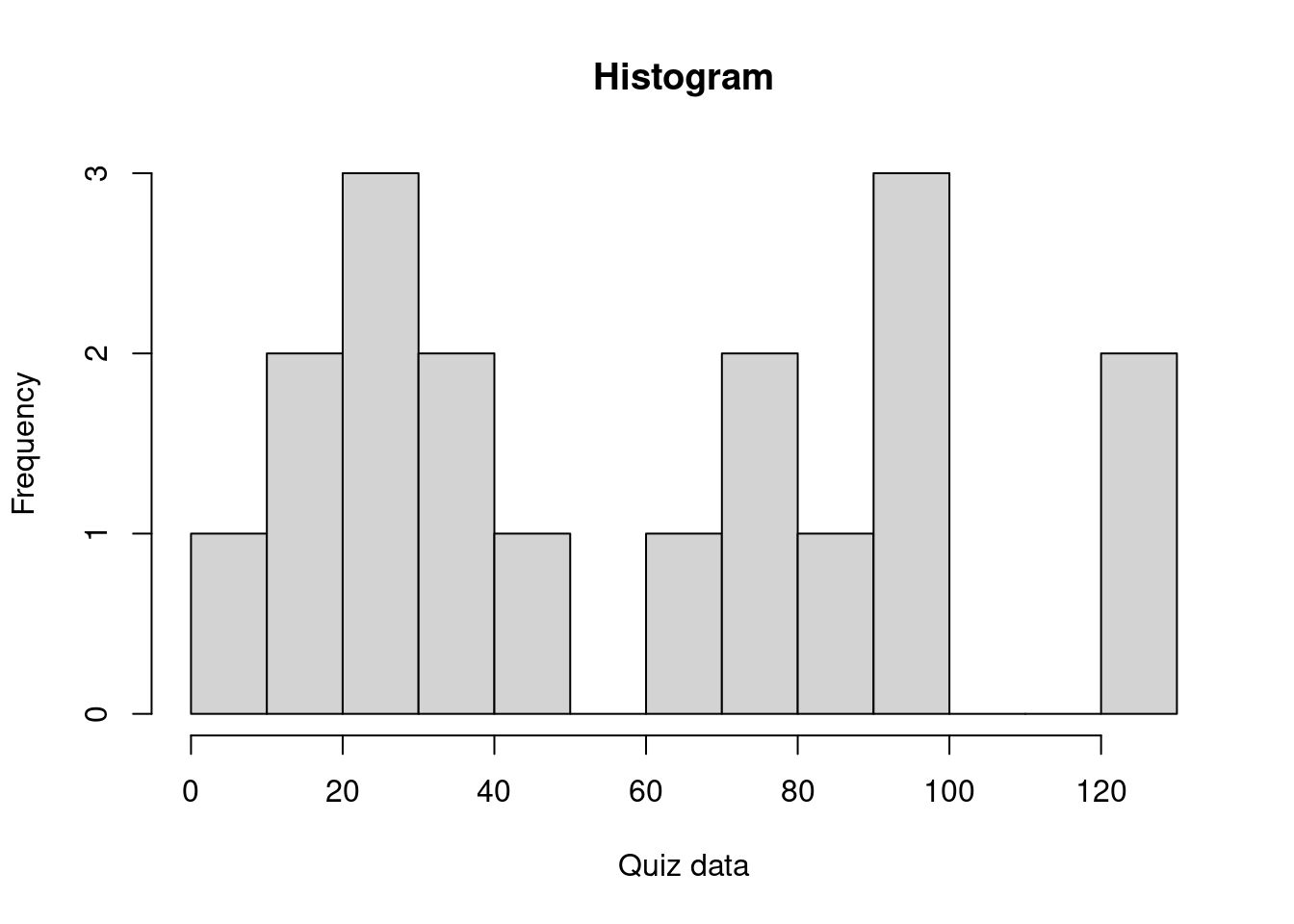
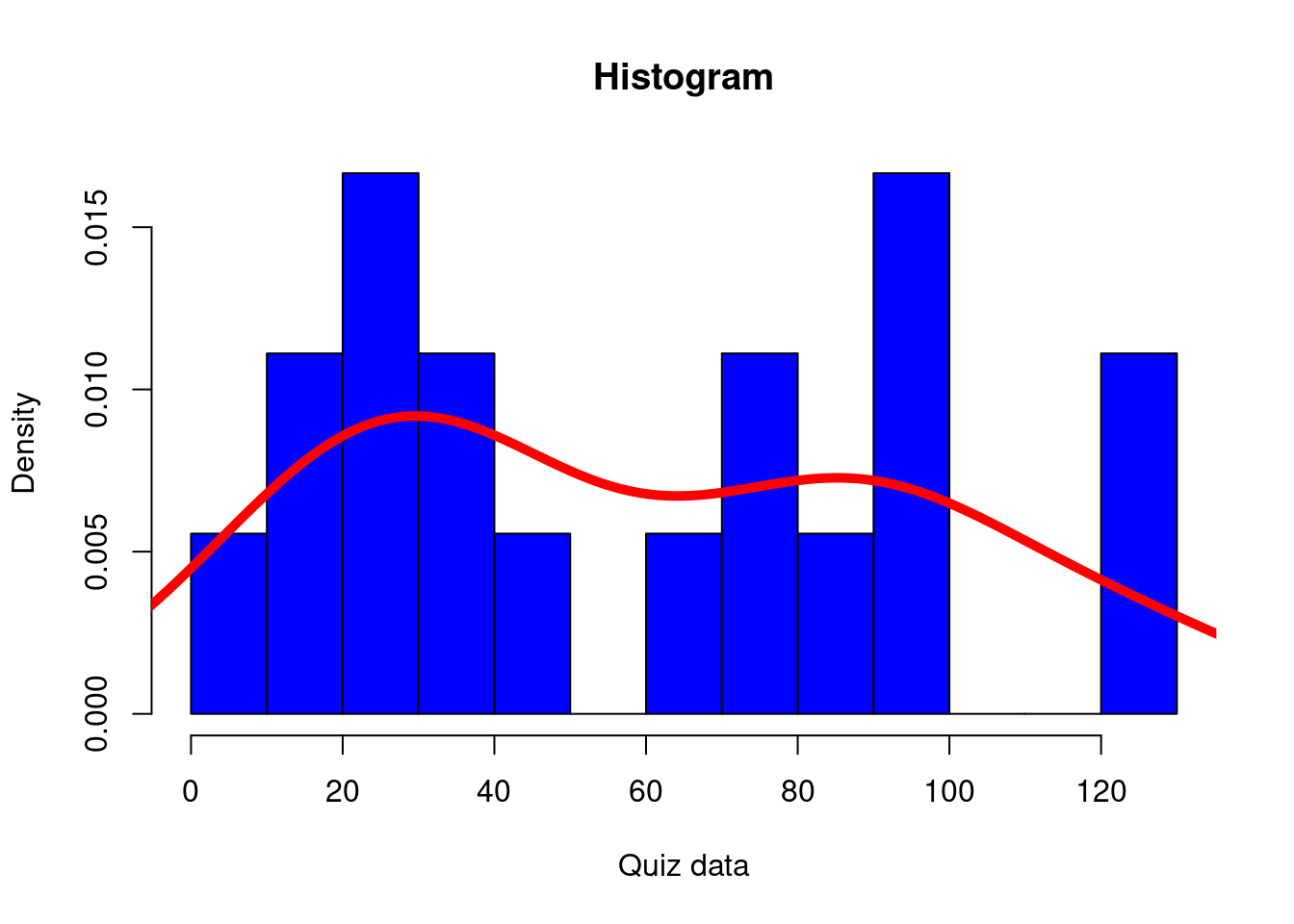
visulization homework

Which of the following has the right R command and the right histogram for the dataset (called quiz_data) from Part 1 (provided below) with a title ‘Histogram’, x-label ‘Quiz data’ and 10 break points?

37,86,79,95,61,93,19,98,121,26,39,11,26,75,29,130,42,8

quiz_data=c(37, 86, 79, 95, 61, 93, 19, 98, 121, 26, 39, 11, 26, 75, 29,130, 42, 8)
hist(quiz_data,breaks=10,main='Histogram',xlab='Quiz data')

You can add options to executable code like this

hist(quiz_data, freq=F, breaks=10, main='Histogram', xlab='Quiz data', col='blue')
lines(density(quiz_data), col='red', lwd=5)

The echo: false option disables the printing of code (only output is displayed).

Footnotes

these are not logical simply some of the mathematical requirements made when estimating least squares.↩︎

Reuse

CC SA BY-NC-ND

Citation

BibTeX citation:

@online{bochman2024,
  author = {Bochman, Oren},
  title = {Practical {Time} {Series} {Analysis}},
  date = {2024-09-17},
  url = {https://orenbochman.github.io/notes/ts-notes/ts01.html},
  langid = {en}
}

For attribution, please cite this work as:

Bochman, Oren. 2024. “Practical Time Series Analysis.” September 17, 2024. https://orenbochman.github.io/notes/ts-notes/ts01.html.