SuperLearner

SuperLearner is an ensambeleing library.
demos
code
r
Author

Oren Bochman

Published

Wednesday, January 10, 2024

This is a SuperLearner demo.

SuperLearner is an ensambeleing library.

This page is taken out of the documentation

Setup dataset

Listing 1: dataset setup
#install.packages(c("SuperLearner","caret", "glmnet", "randomForest", "ggplot2", "RhpcBLASctl","xgboost","ranger"))
data(Boston, package = "MASS")

?MASS::Boston  # Review info on the Boston dataset.>

colSums(is.na(Boston)) # Check for any missing data - looks like we don't have any.
   crim      zn   indus    chas     nox      rm     age     dis     rad     tax 
      0       0       0       0       0       0       0       0       0       0 
ptratio   black   lstat    medv 
      0       0       0       0 
Listing 2: dataset setup
outcome = Boston$medv #Extract our outcome variable from the dataframe.

data = subset(Boston, select = -medv) # Create a dataframe to contain our explanatory variables.
head(data)
crim zn indus chas nox rm age dis rad tax ptratio black lstat
0.00632 18 2.31 0 0.538 6.575 65.2 4.0900 1 296 15.3 396.90 4.98
0.02731 0 7.07 0 0.469 6.421 78.9 4.9671 2 242 17.8 396.90 9.14
0.02729 0 7.07 0 0.469 7.185 61.1 4.9671 2 242 17.8 392.83 4.03
0.03237 0 2.18 0 0.458 6.998 45.8 6.0622 3 222 18.7 394.63 2.94
0.06905 0 2.18 0 0.458 7.147 54.2 6.0622 3 222 18.7 396.90 5.33
0.02985 0 2.18 0 0.458 6.430 58.7 6.0622 3 222 18.7 394.12 5.21
Listing 3: dataset setup
str(data) # Check structure of our dataframe.
'data.frame':   506 obs. of  13 variables:
 $ crim   : num  0.00632 0.02731 0.02729 0.03237 0.06905 ...
 $ zn     : num  18 0 0 0 0 0 12.5 12.5 12.5 12.5 ...
 $ indus  : num  2.31 7.07 7.07 2.18 2.18 2.18 7.87 7.87 7.87 7.87 ...
 $ chas   : int  0 0 0 0 0 0 0 0 0 0 ...
 $ nox    : num  0.538 0.469 0.469 0.458 0.458 0.458 0.524 0.524 0.524 0.524 ...
 $ rm     : num  6.58 6.42 7.18 7 7.15 ...
 $ age    : num  65.2 78.9 61.1 45.8 54.2 58.7 66.6 96.1 100 85.9 ...
 $ dis    : num  4.09 4.97 4.97 6.06 6.06 ...
 $ rad    : int  1 2 2 3 3 3 5 5 5 5 ...
 $ tax    : num  296 242 242 222 222 222 311 311 311 311 ...
 $ ptratio: num  15.3 17.8 17.8 18.7 18.7 18.7 15.2 15.2 15.2 15.2 ...
 $ black  : num  397 397 393 395 397 ...
 $ lstat  : num  4.98 9.14 4.03 2.94 5.33 ...
Listing 4: dataset setup
dim(data) # Review our dimensions.
[1] 506  13
Listing 5: dataset setup
set.seed(1)# Set a seed for reproducibility in this random sampling.

train_obs = sample(nrow(data), 150) # Reduce to a dataset of 150 observations to speed up model fitting.

x_train = data[train_obs, ] # X is our training sample.


x_holdout = data[-train_obs, ] # Create a holdout set for evaluating model performance.
# Note: cross-validation is even better than a single holdout sample.

outcome_bin = as.numeric(outcome > 22) # Create a binary outcome variable: towns in which median home value is > 22,000.

y_train = outcome_bin[train_obs]
y_holdout = outcome_bin[-train_obs]


table(y_train, useNA = "ifany") # Review the outcome variable distribution.
y_train
 0  1 
92 58 

Review available models

Listing 6: model review
library(SuperLearner)

listWrappers() # Review available models.
All prediction algorithm wrappers in SuperLearner:
 [1] "SL.bartMachine"      "SL.bayesglm"         "SL.biglasso"        
 [4] "SL.caret"            "SL.caret.rpart"      "SL.cforest"         
 [7] "SL.earth"            "SL.gam"              "SL.gbm"             
[10] "SL.glm"              "SL.glm.interaction"  "SL.glmnet"          
[13] "SL.ipredbagg"        "SL.kernelKnn"        "SL.knn"             
[16] "SL.ksvm"             "SL.lda"              "SL.leekasso"        
[19] "SL.lm"               "SL.loess"            "SL.logreg"          
[22] "SL.mean"             "SL.nnet"             "SL.nnls"            
[25] "SL.polymars"         "SL.qda"              "SL.randomForest"    
[28] "SL.ranger"           "SL.ridge"            "SL.rpart"           
[31] "SL.rpartPrune"       "SL.speedglm"         "SL.speedlm"         
[34] "SL.step"             "SL.step.forward"     "SL.step.interaction"
[37] "SL.stepAIC"          "SL.svm"              "SL.template"        
[40] "SL.xgboost"         

All screening algorithm wrappers in SuperLearner:
[1] "All"
[1] "screen.corP"           "screen.corRank"        "screen.glmnet"        
[4] "screen.randomForest"   "screen.SIS"            "screen.template"      
[7] "screen.ttest"          "write.screen.template"
Listing 7: model review
SL.glmnet
function (Y, X, newX, family, obsWeights, id, alpha = 1, nfolds = 10, 
    nlambda = 100, useMin = TRUE, loss = "deviance", ...) 
{
    .SL.require("glmnet")
    if (!is.matrix(X)) {
        X <- model.matrix(~-1 + ., X)
        newX <- model.matrix(~-1 + ., newX)
    }
    fitCV <- glmnet::cv.glmnet(x = X, y = Y, weights = obsWeights, 
        lambda = NULL, type.measure = loss, nfolds = nfolds, 
        family = family$family, alpha = alpha, nlambda = nlambda, 
        ...)
    pred <- predict(fitCV, newx = newX, type = "response", s = ifelse(useMin, 
        "lambda.min", "lambda.1se"))
    fit <- list(object = fitCV, useMin = useMin)
    class(fit) <- "SL.glmnet"
    out <- list(pred = pred, fit = fit)
    return(out)
}
<bytecode: 0x648245d66b50>
<environment: namespace:SuperLearner>

Fit individual models

Let’s fit 2 separate models: lasso (sparse, penalized OLS) and random forest. We specify family = binomial() because we are predicting a binary outcome, aka classification. With a continuous outcome we would specify family = gaussian().

Listing 8: fit lasso
set.seed(1) # Set the seed for reproducibility.

sl_lasso = SuperLearner(Y = y_train, X = x_train, family = binomial(),
                        SL.library = "SL.glmnet") # Fit lasso model.
Loading required namespace: glmnet
Listing 9: fit lasso
sl_lasso

Call:  
SuperLearner(Y = y_train, X = x_train, family = binomial(), SL.library = "SL.glmnet") 

                    Risk Coef
SL.glmnet_All 0.08484849    1
Listing 10: fit lasso
names(sl_lasso)
 [1] "call"              "libraryNames"      "SL.library"       
 [4] "SL.predict"        "coef"              "library.predict"  
 [7] "Z"                 "cvRisk"            "family"           
[10] "fitLibrary"        "cvFitLibrary"      "varNames"         
[13] "validRows"         "method"            "whichScreen"      
[16] "control"           "cvControl"         "errorsInCVLibrary"
[19] "errorsInLibrary"   "metaOptimizer"     "env"              
[22] "times"            
Listing 11: fit lasso
sl_lasso$cvRisk[which.min(sl_lasso$cvRisk)]
SL.glmnet_All 
   0.08484849 
Listing 12: fit lasso
str(sl_lasso$fitLibrary$SL.glmnet_All$object, max.level = 1)
List of 12
 $ lambda    : num [1:90] 0.317 0.289 0.263 0.24 0.218 ...
 $ cvm       : num [1:90] 1.34 1.28 1.21 1.16 1.1 ...
 $ cvsd      : num [1:90] 0.0359 0.033 0.0304 0.0292 0.0291 ...
 $ cvup      : num [1:90] 1.38 1.31 1.24 1.18 1.13 ...
 $ cvlo      : num [1:90] 1.31 1.24 1.18 1.13 1.08 ...
 $ nzero     : Named int [1:90] 0 1 1 1 1 1 2 2 2 2 ...
  ..- attr(*, "names")= chr [1:90] "s0" "s1" "s2" "s3" ...
 $ call      : language glmnet::cv.glmnet(x = X, y = Y, weights = obsWeights, lambda = NULL, type.measure = loss,      nfolds = nfolds, f| __truncated__
 $ name      : Named chr "Binomial Deviance"
  ..- attr(*, "names")= chr "deviance"
 $ glmnet.fit:List of 13
  ..- attr(*, "class")= chr [1:2] "lognet" "glmnet"
 $ lambda.min: num 0.0161
 $ lambda.1se: num 0.0652
 $ index     : int [1:2, 1] 33 18
  ..- attr(*, "dimnames")=List of 2
 - attr(*, "class")= chr "cv.glmnet"
Listing 13: fit lasso
sl_rf = SuperLearner(Y = y_train, X = x_train, family = binomial(),
                     SL.library = "SL.ranger")
Loading required namespace: ranger
Listing 14: fit lasso
names(sl_lasso)
 [1] "call"              "libraryNames"      "SL.library"       
 [4] "SL.predict"        "coef"              "library.predict"  
 [7] "Z"                 "cvRisk"            "family"           
[10] "fitLibrary"        "cvFitLibrary"      "varNames"         
[13] "validRows"         "method"            "whichScreen"      
[16] "control"           "cvControl"         "errorsInCVLibrary"
[19] "errorsInLibrary"   "metaOptimizer"     "env"              
[22] "times"            
Listing 15: fit lasso
sl_lasso$cvRisk[which.min(sl_lasso$cvRisk)]
SL.glmnet_All 
   0.08484849 
Listing 16: fit lasso
# Here is the raw glmnet result object:
str(sl_lasso$fitLibrary$SL.glmnet_All$object, max.level = 1)
List of 12
 $ lambda    : num [1:90] 0.317 0.289 0.263 0.24 0.218 ...
 $ cvm       : num [1:90] 1.34 1.28 1.21 1.16 1.1 ...
 $ cvsd      : num [1:90] 0.0359 0.033 0.0304 0.0292 0.0291 ...
 $ cvup      : num [1:90] 1.38 1.31 1.24 1.18 1.13 ...
 $ cvlo      : num [1:90] 1.31 1.24 1.18 1.13 1.08 ...
 $ nzero     : Named int [1:90] 0 1 1 1 1 1 2 2 2 2 ...
  ..- attr(*, "names")= chr [1:90] "s0" "s1" "s2" "s3" ...
 $ call      : language glmnet::cv.glmnet(x = X, y = Y, weights = obsWeights, lambda = NULL, type.measure = loss,      nfolds = nfolds, f| __truncated__
 $ name      : Named chr "Binomial Deviance"
  ..- attr(*, "names")= chr "deviance"
 $ glmnet.fit:List of 13
  ..- attr(*, "class")= chr [1:2] "lognet" "glmnet"
 $ lambda.min: num 0.0161
 $ lambda.1se: num 0.0652
 $ index     : int [1:2, 1] 33 18
  ..- attr(*, "dimnames")=List of 2
 - attr(*, "class")= chr "cv.glmnet"
# Fit random forest.
sl_rf = SuperLearner(Y = y_train, X = x_train, family = binomial(), SL.library = "SL.ranger")

sl_rf

Call:  
SuperLearner(Y = y_train, X = x_train, family = binomial(), SL.library = "SL.ranger") 

                    Risk Coef
SL.ranger_All 0.07620479    1

Fit multiple models

Listing 17: lst fit multiple models
set.seed(1)
sl = SuperLearner(Y = y_train, X = x_train, family = binomial(),
  SL.library = c("SL.mean", "SL.glmnet", "SL.ranger"))

sl

Call:  
SuperLearner(Y = y_train, X = x_train, family = binomial(), SL.library = c("SL.mean",  
    "SL.glmnet", "SL.ranger")) 

                    Risk       Coef
SL.mean_All   0.23773937 0.00000000
SL.glmnet_All 0.08847869 0.02212495
SL.ranger_All 0.07053788 0.97787505
Listing 18: lst fit multiple models
sl$times$everything
   user  system elapsed 
  1.324   0.016   1.346 

Again, the coefficient is how much weight SuperLearner puts on that model in the weighted-average. So if coefficient = 0 it means that model is not used at all. Here we see that random forest is given the most weight, following by lasso.

So we have an automatic ensemble of multiple learners based on the cross-validated performance of those learners, nice!

Predict on new data

Now that we have an ensemble let’s predict back on our holdout dataset and review the results.

Listing 19: predict
# onlySL is set to TRUE so we don't fit algorithms that had weight = 0, saving computation.
pred = predict(sl, x_holdout, onlySL = TRUE)
Loading required namespace: glmnet
Loading required namespace: ranger
Listing 20: predict
# Check the structure of this prediction object.
str(pred)
List of 2
 $ pred           : num [1:356, 1] 0.577 0.891 0.939 0.943 0.853 ...
 $ library.predict: num [1:356, 1:3] 0 0 0 0 0 0 0 0 0 0 ...
Listing 21: predict
# Review the columns of $library.predict.
summary(pred$library.predict)
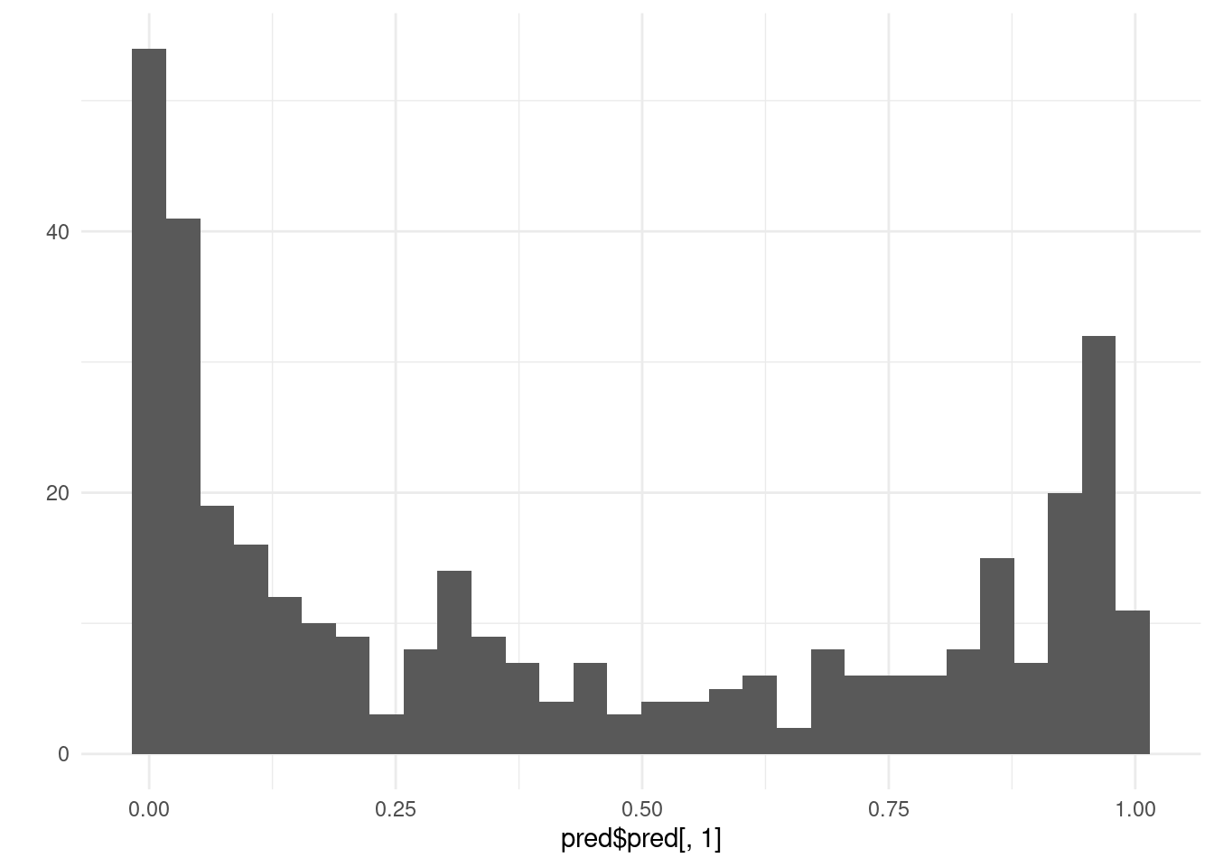
       V1          V2                 V3           
 Min.   :0   Min.   :0.000008   Min.   :0.0002625  
 1st Qu.:0   1st Qu.:0.026812   1st Qu.:0.0484115  
 Median :0   Median :0.310300   Median :0.3057313  
 Mean   :0   Mean   :0.404139   Mean   :0.4124046  
 3rd Qu.:0   3rd Qu.:0.782474   3rd Qu.:0.8181667  
 Max.   :0   Max.   :0.998259   Max.   :0.9980000  
Listing 22: predict
library(ggplot2)
qplot(pred$pred[, 1]) + theme_minimal()
Warning: `qplot()` was deprecated in ggplot2 3.4.0.
`stat_bin()` using `bins = 30`. Pick better value with `binwidth`.

Listing 23: predict
## `stat_bin()` using `bins = 30`. Pick better value with `binwidth`.

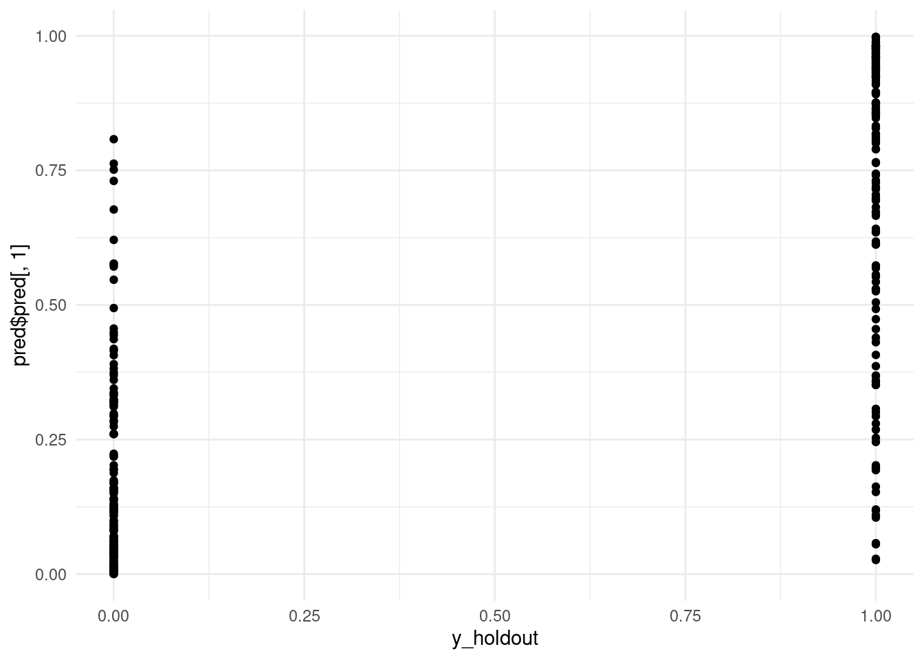
# Scatterplot of original values (0, 1) and predicted values.
# Ideally we would use jitter or slight transparency to deal with overlap.
qplot(y_holdout, pred$pred[, 1]) + theme_minimal()

Listing 24: predict
# Review AUC - Area Under Curve
pred_rocr = ROCR::prediction(pred$pred, y_holdout)
auc = ROCR::performance(pred_rocr, measure = "auc", x.measure = "cutoff")@y.values[[1]]
auc
[1] 0.9443598

Fit ensemble with external cross-validation

What we don’t have yet is an estimate of the performance of the ensemble itself. Right now we are just hopeful that the ensemble weights are successful in improving over the best single algorithm.

In order to estimate the performance of the SuperLearner ensemble we need an “external” layer of cross-validation, also called nested cross-validation. We generate a separate holdout sample that we don’t use to fit the SuperLearner, which allows it to be a good estimate of the SuperLearner’s performance on unseen data. Typically we would run 10 or 20-fold external cross-validation, but even 5-fold is reasonable.

Another nice result is that we get standard errors on the performance of the individual algorithms and can compare them to the SuperLearner.

set.seed(1)

# Don't have timing info for the CV.SuperLearner unfortunately.
# So we need to time it manually.

system.time({
  # This will take about 2x as long as the previous SuperLearner.
  cv_sl = CV.SuperLearner(Y = y_train, X = x_train, family = binomial(),
                          # For a real analysis we would use V = 10.
                          V = 3,
                          SL.library = c("SL.mean", "SL.glmnet", "SL.ranger"))
})
   user  system elapsed 
  5.235   0.143   5.400 
# We run summary on the cv_sl object rather than simply printing the object.
summary(cv_sl)

Call:  
CV.SuperLearner(Y = y_train, X = x_train, V = 3, family = binomial(), SL.library = c("SL.mean",  
    "SL.glmnet", "SL.ranger")) 

Risk is based on: Mean Squared Error

All risk estimates are based on V =  3 

     Algorithm      Ave       se      Min      Max
 Super Learner 0.074388 0.011392 0.064595 0.084275
   Discrete SL 0.077512 0.011293 0.067146 0.086532
   SL.mean_All 0.251267 0.010352 0.228500 0.289600
 SL.glmnet_All 0.081595 0.014502 0.072729 0.095522
 SL.ranger_All 0.077512 0.011293 0.067146 0.086532
# Review the distribution of the best single learner as external CV folds.
table(simplify2array(cv_sl$whichDiscreteSL))

SL.ranger_All 
            3 
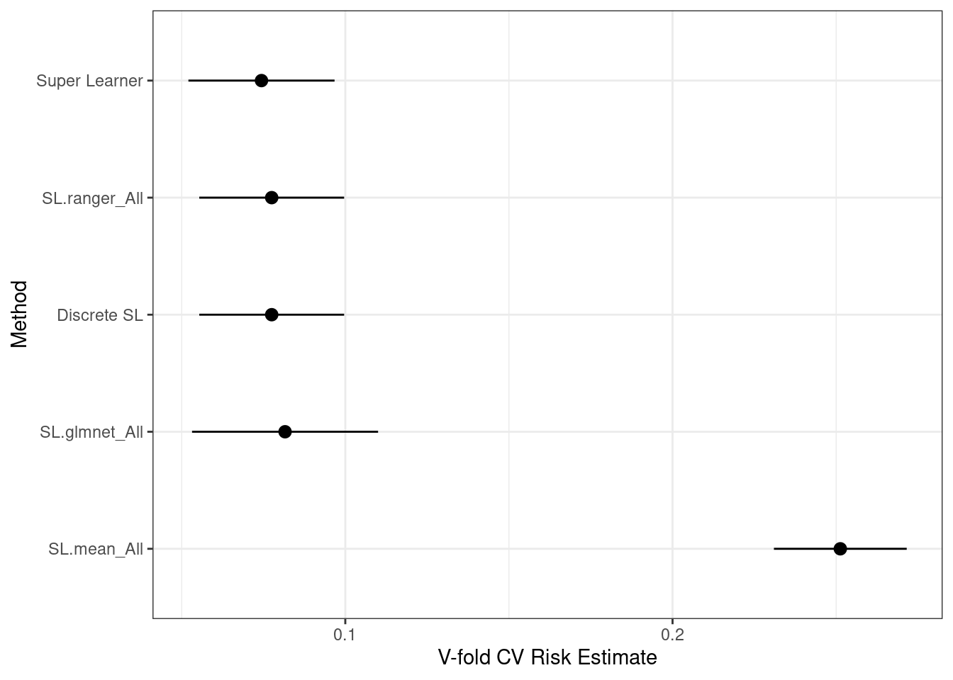
# Plot the performance with 95% CIs (use a better ggplot theme).
plot(cv_sl) + theme_bw()

ggsave("SuperLearner.png")
Saving 7 x 5 in image

Customize a model hyperparameter

Hyperparameters are the configuration settings for an algorithm. OLS has no hyperparameters but essentially every other algorithm does.

There are two ways to customize a hyperparameter: make a new learner function, or use create.Learner().

Let’s make a variant of random forest that fits more trees, which may increase our accuracy and can’t hurt it (outside of small random variation).

# Review the function argument defaults at the top.
SL.ranger
function (Y, X, newX, family, obsWeights, num.trees = 500, mtry = floor(sqrt(ncol(X))), 
    write.forest = TRUE, probability = family$family == "binomial", 
    min.node.size = ifelse(family$family == "gaussian", 5, 1), 
    replace = TRUE, sample.fraction = ifelse(replace, 1, 0.632), 
    num.threads = 1, verbose = T, ...) 
{
    .SL.require("ranger")
    if (family$family == "binomial") {
        Y = as.factor(Y)
    }
    if (is.matrix(X)) {
        X = data.frame(X)
    }
    fit <- ranger::ranger(`_Y` ~ ., data = cbind(`_Y` = Y, X), 
        num.trees = num.trees, mtry = mtry, min.node.size = min.node.size, 
        replace = replace, sample.fraction = sample.fraction, 
        case.weights = obsWeights, write.forest = write.forest, 
        probability = probability, num.threads = num.threads, 
        verbose = verbose)
    pred <- predict(fit, data = newX)$predictions
    if (family$family == "binomial") {
        pred = pred[, "1"]
    }
    fit <- list(object = fit, verbose = verbose)
    class(fit) <- c("SL.ranger")
    out <- list(pred = pred, fit = fit)
    return(out)
}
<bytecode: 0x5f8eb7044c60>
<environment: namespace:SuperLearner>
# Create a new function that changes just the ntree argument.
# (We could do this in a single line.)
# "..." means "all other arguments that were sent to the function"
SL.rf.better = function(...) {
  SL.randomForest(..., num.trees = 1000)
}

set.seed(1)

# Fit the CV.SuperLearner.
# We use V = 3 to save computation time; for a real analysis use V = 10 or 20.
cv_sl = CV.SuperLearner(Y = y_train, X = x_train, family = binomial(), V = 3,
                        SL.library = c("SL.mean", "SL.glmnet", "SL.rf.better", "SL.ranger"))
Loading required namespace: glmnet
Loading required namespace: randomForest
Loading required namespace: ranger
# Review results.
summary(cv_sl)

Call:  
CV.SuperLearner(Y = y_train, X = x_train, V = 3, family = binomial(), SL.library = c("SL.mean",  
    "SL.glmnet", "SL.rf.better", "SL.ranger")) 

Risk is based on: Mean Squared Error

All risk estimates are based on V =  3 

        Algorithm      Ave       se      Min      Max
    Super Learner 0.075382 0.011316 0.066279 0.085697
      Discrete SL 0.078154 0.011304 0.065446 0.090042
      SL.mean_All 0.251267 0.010352 0.228500 0.289600
    SL.glmnet_All 0.080752 0.014631 0.076383 0.088697
 SL.rf.better_All 0.078075 0.011301 0.065446 0.089805
    SL.ranger_All 0.080011 0.011452 0.066660 0.090042
# Customize the defaults for random forest.
learners = create.Learner("SL.ranger", params = list(num.trees = 1000))

# Look at the object.
learners
$grid
NULL

$names
[1] "SL.ranger_1"

$base_learner
[1] "SL.ranger"

$params
$params$num.trees
[1] 1000
# List the functions that were created
learners$names
[1] "SL.ranger_1"
# Review the code that was automatically generated for the function.
# Notice that it's exactly the same as the function we made manually.
SL.ranger_1
function (...) 
SL.ranger(..., num.trees = 1000)
set.seed(1)

# Fit the CV.SuperLearner.
# We use V = 3 to save computation time; for a real analysis use V = 10 or 20.
cv_sl = CV.SuperLearner(Y = y_train, X = x_train, family = binomial(),
                        V = 3,
                        SL.library = c("SL.mean", "SL.glmnet", learners$names, "SL.ranger"))

# Review results.
summary(cv_sl)

Call:  
CV.SuperLearner(Y = y_train, X = x_train, V = 3, family = binomial(), SL.library = c("SL.mean",  
    "SL.glmnet", learners$names, "SL.ranger")) 

Risk is based on: Mean Squared Error

All risk estimates are based on V =  3 

       Algorithm      Ave       se      Min      Max
   Super Learner 0.073994 0.010872 0.065059 0.083029
     Discrete SL 0.077243 0.011034 0.065593 0.089188
     SL.mean_All 0.251267 0.010352 0.228500 0.289600
   SL.glmnet_All 0.080148 0.013766 0.076383 0.087422
 SL.ranger_1_All 0.077687 0.011077 0.065593 0.089188
   SL.ranger_All 0.077231 0.011078 0.065675 0.089071

Test algorithm with multiple hyperparameter settings

The performance of an algorithm varies based on its hyperparamters, which again are its configuration settings. Some algorithms may not vary much, and others might have far better or worse performance for certain settings. Often we focus our attention on 1 or 2 hyperparameters for a given algorithm because they are the most important ones.

For random forest there are two particularly important hyperparameters: mtry and maximum leaf nodes. Mtry is how many features are randomly chosen within each decision tree node - in other words, each time the tree considers making a split. Maximum leaf nodes controls how complex each tree can get.

Let’s try 3 different mtry options.

# sqrt(p) is the default value of mtry for classification.
floor(sqrt(ncol(x_train)))
[1] 3
## [1] 3
# Let's try 3 multiplies of this default: 0.5, 1, and 2.
(mtry_seq = floor(sqrt(ncol(x_train)) * c(0.5, 1, 2)))
[1] 1 3 7
## [1] 1 3 7
learners = create.Learner("SL.ranger", tune = list(mtry = mtry_seq))

# Review the resulting object
learners
$grid
  mtry
1    1
2    3
3    7

$names
[1] "SL.ranger_1" "SL.ranger_2" "SL.ranger_3"

$base_learner
[1] "SL.ranger"

$params
list()
SL.ranger_1
function (...) 
SL.ranger(..., mtry = 1)
SL.ranger_2
function (...) 
SL.ranger(..., mtry = 3)
SL.ranger_3
function (...) 
SL.ranger(..., mtry = 7)
set.seed(1)

# Fit the CV.SuperLearner.
# We use V = 3 to save computation time; for a real analysis use V = 10 or 20.
cv_sl = CV.SuperLearner(Y = y_train, X = x_train, 
                        family = binomial(), V = 3, 
                        SL.library = c("SL.mean", "SL.glmnet", learners$names, "SL.ranger"))
Loading required namespace: glmnet
Loading required namespace: ranger
# Review results.
summary(cv_sl)

Call:  
CV.SuperLearner(Y = y_train, X = x_train, V = 3, family = binomial(), SL.library = c("SL.mean",  
    "SL.glmnet", learners$names, "SL.ranger")) 

Risk is based on: Mean Squared Error

All risk estimates are based on V =  3 

       Algorithm      Ave       se      Min      Max
   Super Learner 0.067516 0.011105 0.056210 0.081632
     Discrete SL 0.071761 0.011897 0.057843 0.092998
     SL.mean_All 0.251267 0.010352 0.228500 0.289600
   SL.glmnet_All 0.078227 0.015002 0.070147 0.087422
 SL.ranger_1_All 0.102194 0.011360 0.089415 0.111369
 SL.ranger_2_All 0.078006 0.011196 0.064298 0.093298
 SL.ranger_3_All 0.071761 0.011897 0.057843 0.092998
   SL.ranger_All 0.078469 0.011270 0.065888 0.089501

We see here that mtry = 7 performed a little bit better than mtry = 1 or mtry = 3, although the difference is not significant. If we used more data and more cross-validation folds we might see more drastic differences. A higher mtry does better when a small percentage of variables are predictive of the outcome, because it gives each tree a better chance of finding a useful variable.

Note that SL.ranger and SL.ranger_2 have the same settings, and their performance is very similar - statistically a tie. It’s not exactly equivalent due to random variation in the two forests.

A key difference with SuperLearner over caret or other frameworks is that we are not trying to choose the single best hyperparameter or model. Instead, we usually want the best weighted average. So we are including all of the different settings in our SuperLearner, and we may choose a weighted average that includes the same model multiple times but with different settings. That can give us better performance than choosing only the single best settings for a given algorithm, which has some random noise in any case.

Multicore parallelization SuperLearner makes it easy to use multiple CPU cores on your computer to speed up the calculations. We first need to setup R for multiple cores, then tell CV.SuperLearner to divide its computations across those cores.

There are two ways to use multiple cores in R: the “multicore” system and the “snow” system. Windows only supports the “snow” system, which is more difficult to use, whereas macOS and Linux can use either one.

First we show the “multicore” system version:

# Setup parallel computation - use all cores on our computer.
(num_cores = RhpcBLASctl::get_num_cores())
[1] 8
# Use 2 of those cores for parallel SuperLearner.
# Replace "2" with "num_cores" (without quotes) to use all cores.
options(mc.cores = 2)

# Check how many parallel workers we are using (on macOS/Linux).
getOption("mc.cores")
[1] 2
# We need to set a different type of seed that works across cores.
# Otherwise the other cores will go rogue and we won't get repeatable results.
# This version is for the "multicore" parallel system in R.
set.seed(1, "L'Ecuyer-CMRG")

# While this is running check CPU using in Activity Monitor / Task Manager.
system.time({
  cv_sl = CV.SuperLearner(Y = y_train, X = x_train, family = binomial(),
                          # For a real analysis we would use V = 10.
                          V = 3,
                          parallel = "multicore",
                          SL.library = c("SL.mean", "SL.glmnet", learners$names, "SL.ranger"))
})
Loading required namespace: parallel
   user  system elapsed 
  1.918   0.272   4.835 
# Review results.
summary(cv_sl)

Call:  
CV.SuperLearner(Y = y_train, X = x_train, V = 3, family = binomial(), SL.library = c("SL.mean",  
    "SL.glmnet", learners$names, "SL.ranger"), parallel = "multicore") 

Risk is based on: Mean Squared Error

All risk estimates are based on V =  3 

       Algorithm      Ave        se      Min      Max
   Super Learner 0.089148 0.0149989 0.053080 0.107932
     Discrete SL 0.097739 0.0174582 0.059888 0.125348
     SL.mean_All 0.242600 0.0095617 0.226900 0.260500
   SL.glmnet_All 0.103421 0.0164995 0.059888 0.125348
 SL.ranger_1_All 0.093995 0.0107773 0.070773 0.106005
 SL.ranger_2_All 0.080877 0.0120526 0.053931 0.099784
 SL.ranger_3_All 0.084269 0.0142342 0.044643 0.107982
   SL.ranger_All 0.081619 0.0120937 0.052445 0.101650

Here is the “snow” equivalent:

# Make a snow cluster
# Again, replace 2 with num_cores to use all available cores.
cluster = parallel::makeCluster(2)

# Check the cluster object.
cluster
socket cluster with 2 nodes on host 'localhost'
# Load the SuperLearner package on all workers so they can find
# SuperLearner::All(), the default screening function which keeps all variables.
parallel::clusterEvalQ(cluster, library(SuperLearner))
[[1]]
 [1] "SuperLearner" "gam"          "foreach"      "splines"      "nnls"        
 [6] "stats"        "graphics"     "grDevices"    "utils"        "datasets"    
[11] "methods"      "base"        

[[2]]
 [1] "SuperLearner" "gam"          "foreach"      "splines"      "nnls"        
 [6] "stats"        "graphics"     "grDevices"    "utils"        "datasets"    
[11] "methods"      "base"        
# We need to explictly export our custom learner functions to the workers.
parallel::clusterExport(cluster, learners$names)

# We need to set a different type of seed that works across cores.
# This version is for SNOW parallelization.
# Otherwise the other cores will go rogue and we won't get repeatable results.
parallel::clusterSetRNGStream(cluster, 1)

# While this is running check CPU using in Activity Monitor / Task Manager.
system.time({
  cv_sl = CV.SuperLearner(Y = y_train, X = x_train, family = binomial(),
                          # For a real analysis we would use V = 10.
                          V = 3,
                          parallel = cluster,
                          SL.library = c("SL.mean", "SL.glmnet", learners$names, "SL.ranger"))
})
   user  system elapsed 
  0.007   0.000   5.484 
# Review results.
summary(cv_sl)

Call:  
CV.SuperLearner(Y = y_train, X = x_train, V = 3, family = binomial(), SL.library = c("SL.mean",  
    "SL.glmnet", learners$names, "SL.ranger"), parallel = cluster) 

Risk is based on: Mean Squared Error

All risk estimates are based on V =  3 

       Algorithm      Ave        se      Min      Max
   Super Learner 0.074781 0.0141069 0.063216 0.091040
     Discrete SL 0.070968 0.0132823 0.063216 0.079742
     SL.mean_All 0.238600 0.0091846 0.229300 0.246100
   SL.glmnet_All 0.097299 0.0185871 0.072560 0.120085
 SL.ranger_1_All 0.097233 0.0113360 0.093720 0.101704
 SL.ranger_2_All 0.076001 0.0119746 0.068762 0.082897
 SL.ranger_3_All 0.070968 0.0132823 0.063216 0.079742
   SL.ranger_All 0.076301 0.0118938 0.069590 0.082703
# Stop the cluster workers now that we're done.
parallel::stopCluster(cluster)

If we want to use multiple cores for normal SuperLearner, not CV.SuperLearner (i.e. external cross-validation to estimate performance), we need to change the function name to mcSuperLearner (“multicore” version) or snowSuperLearner (“snow” version).

First the “multicore” version (won’t be parallel on Windows):

# Set multicore compatible seed.
set.seed(1, "L'Ecuyer-CMRG")

# Fit the SuperLearner.
(sl = mcSuperLearner(Y = y_train, X = x_train, family = binomial(),
                    SL.library = c("SL.mean", "SL.glmnet", learners$names, "SL.ranger")))

Call:  
mcSuperLearner(Y = y_train, X = x_train, family = binomial(), SL.library = c("SL.mean",  
    "SL.glmnet", learners$names, "SL.ranger")) 

                      Risk       Coef
SL.mean_All     0.24253498 0.00000000
SL.glmnet_All   0.09181320 0.02471622
SL.ranger_1_All 0.09498042 0.00000000
SL.ranger_2_All 0.07428239 0.00000000
SL.ranger_3_All 0.07102085 0.92627825
SL.ranger_All   0.07388773 0.04900552
# We see the time is reduced over our initial single-core superlearner.
sl$times$everything
   user  system elapsed 
  2.749   0.358   1.888 

Now the “snow” version, which should be parallel on all operating systems.

# Make a snow cluster
# Reminder: change "2" to "num_cores" (without quotes) to use all available cores.
(cluster = parallel::makeCluster(2))
socket cluster with 2 nodes on host 'localhost'
## socket cluster with 2 nodes on host 'localhost'
# Load the SuperLearner package on all workers so they can find
# SuperLearner::All(), the default screening function which keeps all variables.
parallel::clusterEvalQ(cluster, library(SuperLearner))
[[1]]
 [1] "SuperLearner" "gam"          "foreach"      "splines"      "nnls"        
 [6] "stats"        "graphics"     "grDevices"    "utils"        "datasets"    
[11] "methods"      "base"        

[[2]]
 [1] "SuperLearner" "gam"          "foreach"      "splines"      "nnls"        
 [6] "stats"        "graphics"     "grDevices"    "utils"        "datasets"    
[11] "methods"      "base"        
# We need to explictly export our custom learner functions to the workers.
parallel::clusterExport(cluster, learners$names)

# We need to set a different type of seed that works across cores.
# This version is for SNOW parallelization.
# Otherwise the other cores will go rogue and we won't get repeatable results.
parallel::clusterSetRNGStream(cluster, 1)

# Fit the SuperLearner.
(sl = snowSuperLearner(Y = y_train, X = x_train, family = binomial(),
                      cluster = cluster,
                      SL.library = c("SL.mean", "SL.glmnet", learners$names, "SL.ranger")))

Call:  
snowSuperLearner(cluster = cluster, Y = y_train, X = x_train, family = binomial(),  
    SL.library = c("SL.mean", "SL.glmnet", learners$names, "SL.ranger")) 

                      Risk       Coef
SL.mean_All     0.23878189 0.00000000
SL.glmnet_All   0.08486885 0.13188912
SL.ranger_1_All 0.09253551 0.00000000
SL.ranger_2_All 0.07253553 0.01627661
SL.ranger_3_All 0.06974784 0.85183427
SL.ranger_All   0.07397735 0.00000000
# We see the time is reduced over our initial single-core superlearner.
sl$times$everything
   user  system elapsed 
  0.356   0.036   2.624 

SuperLearner also supports running across multiple computers at a time, called “multi-node” or “cluster” computing. We will skip that for now.

Weight distribution for SuperLearner

The weights or coefficients of the SuperLearner are stochastic - they will change as the data changes. So we don’t necessarily trust a given set of weights as being the “true” weights, but when we use CV.SuperLearner we at least have multiple samples from the distribution of the weights.

We can write a little function to extract the weights at each CV.SuperLearner iteration and summarize the distribution of those weights. This may be added to the SuperLearner package sometime in the future.

# Review meta-weights (coefficients) from a CV.SuperLearner object
review_weights = function(cv_sl) {
  meta_weights = coef(cv_sl)
  means = colMeans(meta_weights)
  sds = apply(meta_weights, MARGIN = 2,  FUN = sd)
  mins = apply(meta_weights, MARGIN = 2, FUN = min)
  maxs = apply(meta_weights, MARGIN = 2, FUN = max)
  # Combine the stats into a single matrix.
  sl_stats = cbind("mean(weight)" = means, "sd" = sds, "min" = mins, "max" = maxs)
  # Sort by decreasing mean weight.
  sl_stats[order(sl_stats[, 1], decreasing = TRUE), ]
}

print(review_weights(cv_sl), digits = 3)
                mean(weight)     sd   min   max
SL.ranger_3_All       0.6907 0.2955 0.411 1.000
SL.glmnet_All         0.2588 0.2295 0.000 0.437
SL.ranger_2_All       0.0504 0.0874 0.000 0.151
SL.mean_All           0.0000 0.0000 0.000 0.000
SL.ranger_1_All       0.0000 0.0000 0.000 0.000
SL.ranger_All         0.0000 0.0000 0.000 0.000

Notice that in this case the ensemble never uses the mean nor the randomForest with mtry = 1. Also the LASSO (glmnet) was only used on a subset of the folds. Adding multiple configurations of randomForest was helpful because mtry = 7 was used. However, based on the minimum column we can see that no algorithm was used every single time.

We recommend reviewing the weight distribution for any SuperLearner project to better understand which algorithms are chosen for the ensemble.

Feature selection (screening)

When datasets have many covariates our algorithms may benefit from first choosing a subset of available covariates, a step called feature selection. Then we pass only those variables to the modeling algorithm, and it may be less likely to overfit to variables that are not related to the outcome.

Let’s revisit listWrappers() and check out the bottom section.

listWrappers()
All prediction algorithm wrappers in SuperLearner:
 [1] "SL.bartMachine"      "SL.bayesglm"         "SL.biglasso"        
 [4] "SL.caret"            "SL.caret.rpart"      "SL.cforest"         
 [7] "SL.earth"            "SL.gam"              "SL.gbm"             
[10] "SL.glm"              "SL.glm.interaction"  "SL.glmnet"          
[13] "SL.ipredbagg"        "SL.kernelKnn"        "SL.knn"             
[16] "SL.ksvm"             "SL.lda"              "SL.leekasso"        
[19] "SL.lm"               "SL.loess"            "SL.logreg"          
[22] "SL.mean"             "SL.nnet"             "SL.nnls"            
[25] "SL.polymars"         "SL.qda"              "SL.randomForest"    
[28] "SL.ranger"           "SL.ridge"            "SL.rpart"           
[31] "SL.rpartPrune"       "SL.speedglm"         "SL.speedlm"         
[34] "SL.step"             "SL.step.forward"     "SL.step.interaction"
[37] "SL.stepAIC"          "SL.svm"              "SL.template"        
[40] "SL.xgboost"         

All screening algorithm wrappers in SuperLearner:
[1] "All"
[1] "screen.corP"           "screen.corRank"        "screen.glmnet"        
[4] "screen.randomForest"   "screen.SIS"            "screen.template"      
[7] "screen.ttest"          "write.screen.template"
# Review code for corP, which is based on univariate correlation.
screen.corP
function (Y, X, family, obsWeights, id, method = "pearson", minPvalue = 0.1, 
    minscreen = 2, ...) 
{
    listp <- apply(X, 2, function(x, Y, method) {
        ifelse(var(x) <= 0, 1, cor.test(x, y = Y, method = method)$p.value)
    }, Y = Y, method = method)
    whichVariable <- (listp <= minPvalue)
    if (sum(whichVariable) < minscreen) {
        warning("number of variables with p value less than minPvalue is less than minscreen")
        whichVariable[rank(listp) <= minscreen] <- TRUE
    }
    return(whichVariable)
}
<bytecode: 0x60a974ffbef0>
<environment: namespace:SuperLearner>
set.seed(1)

# Fit the SuperLearner.
# We need to use list() instead of c().
cv_sl = CV.SuperLearner(Y = y_train, X = x_train, family = binomial(),
                        # For a real analysis we would use V = 10.
                        V = 3,
                        parallel = "multicore",
                        SL.library = list("SL.mean", "SL.glmnet", c("SL.glmnet", "screen.corP")))
summary(cv_sl)

Call:  
CV.SuperLearner(Y = y_train, X = x_train, V = 3, family = binomial(), SL.library = list("SL.mean",  
    "SL.glmnet", c("SL.glmnet", "screen.corP")), parallel = "multicore") 

Risk is based on: Mean Squared Error

All risk estimates are based on V =  3 

             Algorithm     Ave        se      Min     Max
         Super Learner 0.10463 0.0168593 0.065549 0.12602
           Discrete SL 0.10492 0.0170909 0.066405 0.12602
           SL.mean_All 0.24260 0.0095617 0.226900 0.26050
         SL.glmnet_All 0.10492 0.0170909 0.066405 0.12602
 SL.glmnet_screen.corP 0.10392 0.0163746 0.066405 0.12303

We see a small performance boost by first screening by univarate correlation with our outcome, and only keeping variables with a p-value less than 0.10. Try using some of the other screening algorithms as they may do even better for a particular dataset.

Optimize for AUC

For binary prediction we are typically trying to maximize AUC, which can be the best performance metric when our outcome variable has some imbalance. In other words, we don’t have exactly 50% 1s and 50% 0s in our outcome. Our SuperLearner is not targeting AUC by default, but it can if we tell it to by specifying our method.

set.seed(1)

cv_sl = CV.SuperLearner(Y = y_train, X = x_train, family = binomial(),
                        # For a real analysis we would use V = 10.
                        V = 3,
                        method = "method.AUC",
                        SL.library = list("SL.mean", "SL.glmnet", c("SL.glmnet", "screen.corP")))
Loading required package: cvAUC
## Loading required package: cvAUC
summary(cv_sl)

Call:  
CV.SuperLearner(Y = y_train, X = x_train, V = 3, family = binomial(), SL.library = list("SL.mean",  
    "SL.glmnet", c("SL.glmnet", "screen.corP")), method = "method.AUC") 

Risk is based on: Area under ROC curve (AUC)

All risk estimates are based on V =  3 

             Algorithm     Ave se     Min     Max
         Super Learner 0.92045 NA 0.89372 0.95429
           Discrete SL 0.91989 NA 0.89372 0.95429
           SL.mean_All 0.50000 NA 0.50000 0.50000
         SL.glmnet_All 0.92322 NA 0.89372 0.95429
 SL.glmnet_screen.corP 0.91989 NA 0.89372 0.95429

This conveniently shows us the AUC for each algorithm without us having to calculate it manually. But we aren’t getting SEs sadly.

Another important optimizer to consider is negative log likelihood, which is intended for binary outcomes and will often work better than NNLS (the default). This is specified by method = “NNloglik”.

XGBoost hyperparameter exploration

XGBoost is a version of GBM that is even faster and has some extra settings. GBM’s adaptivity is determined by its configuration, so we want to thoroughly test a wide range of configurations for any given problem. Let’s do 27 now. This will take a good amount of time (~7 minutes on my computer) so we need to at least use multiple cores, if not multiple computers.

# 3 * 3 * 3 = 27 different configurations.
# For a real analysis we would do 100, 500, or 1000 trees - this is just a demo.
tune = list(ntrees = c(10, 20, 50),
            max_depth = 1:3,
            shrinkage = c(0.001, 0.01, 0.1))

# Set detailed names = T so we can see the configuration for each function.
# Also shorten the name prefix.
learners = create.Learner("SL.xgboost", tune = tune, detailed_names = TRUE, name_prefix = "xgb")

# 27 configurations - not too shabby.
length(learners$names)
[1] 27
learners$names
 [1] "xgb_10_1_0.001" "xgb_20_1_0.001" "xgb_50_1_0.001" "xgb_10_2_0.001"
 [5] "xgb_20_2_0.001" "xgb_50_2_0.001" "xgb_10_3_0.001" "xgb_20_3_0.001"
 [9] "xgb_50_3_0.001" "xgb_10_1_0.01"  "xgb_20_1_0.01"  "xgb_50_1_0.01" 
[13] "xgb_10_2_0.01"  "xgb_20_2_0.01"  "xgb_50_2_0.01"  "xgb_10_3_0.01" 
[17] "xgb_20_3_0.01"  "xgb_50_3_0.01"  "xgb_10_1_0.1"   "xgb_20_1_0.1"  
[21] "xgb_50_1_0.1"   "xgb_10_2_0.1"   "xgb_20_2_0.1"   "xgb_50_2_0.1"  
[25] "xgb_10_3_0.1"   "xgb_20_3_0.1"   "xgb_50_3_0.1"  
# Confirm we have multiple cores configured. This should be > 1.
getOption("mc.cores")
[1] 2
# Remember to set multicore-compatible seed.
set.seed(1, "L'Ecuyer-CMRG")

# Fit the CV.SuperLearner.
system.time({
  cv_sl = CV.SuperLearner(Y = y_train, X = x_train, family = binomial(),
                          # For a real analysis we would use V = 10.
                          V = 3,
                          parallel = "multicore",
                          SL.library = c("SL.mean", "SL.glmnet", learners$names, "SL.ranger"))
})
   user  system elapsed 
333.391   0.667  48.655 
# Review results.
summary(cv_sl)

Call:  
CV.SuperLearner(Y = y_train, X = x_train, V = 3, family = binomial(), SL.library = c("SL.mean",  
    "SL.glmnet", learners$names, "SL.ranger"), parallel = "multicore") 

Risk is based on: Mean Squared Error

All risk estimates are based on V =  3 

          Algorithm      Ave         se      Min     Max
      Super Learner 0.089735 0.01523004 0.052813 0.11879
        Discrete SL 0.095907 0.01699764 0.064775 0.12535
        SL.mean_All 0.242600 0.00956173 0.226900 0.26050
      SL.glmnet_All 0.104150 0.01673952 0.064775 0.12535
 xgb_10_1_0.001_All 0.247864 0.00022090 0.247406 0.24828
 xgb_20_1_0.001_All 0.245773 0.00043925 0.244861 0.24661
 xgb_50_1_0.001_All 0.239599 0.00103601 0.237065 0.24182
 xgb_10_2_0.001_All 0.247864 0.00022090 0.247406 0.24828
 xgb_20_2_0.001_All 0.245773 0.00043925 0.244861 0.24661
 xgb_50_2_0.001_All 0.239599 0.00103601 0.237065 0.24182
 xgb_10_3_0.001_All 0.247864 0.00022090 0.247406 0.24828
 xgb_20_3_0.001_All 0.245773 0.00043925 0.244861 0.24661
 xgb_50_3_0.001_All 0.239599 0.00103601 0.237065 0.24182
  xgb_10_1_0.01_All 0.229984 0.00200462 0.224800 0.23455
  xgb_20_1_0.01_All 0.213539 0.00380533 0.203477 0.22257
  xgb_50_1_0.01_All 0.179899 0.00791583 0.154434 0.20141
  xgb_10_2_0.01_All 0.229984 0.00200462 0.224800 0.23455
  xgb_20_2_0.01_All 0.213539 0.00380533 0.203477 0.22257
  xgb_50_2_0.01_All 0.179899 0.00791583 0.154434 0.20141
  xgb_10_3_0.01_All 0.229984 0.00200462 0.224800 0.23455
  xgb_20_3_0.01_All 0.213539 0.00380533 0.203477 0.22257
  xgb_50_3_0.01_All 0.179899 0.00791583 0.154434 0.20141
   xgb_10_1_0.1_All 0.149806 0.01102873 0.113512 0.18562
   xgb_20_1_0.1_All 0.138650 0.01162345 0.093478 0.18195
   xgb_50_1_0.1_All 0.139119 0.01173685 0.092681 0.18077
   xgb_10_2_0.1_All 0.149806 0.01102873 0.113512 0.18562
   xgb_20_2_0.1_All 0.138650 0.01162345 0.093478 0.18195
   xgb_50_2_0.1_All 0.139119 0.01173685 0.092681 0.18077
   xgb_10_3_0.1_All 0.149806 0.01102873 0.113512 0.18562
   xgb_20_3_0.1_All 0.138650 0.01162345 0.093478 0.18195
   xgb_50_3_0.1_All 0.139119 0.01173685 0.092681 0.18077
      SL.ranger_All 0.079853 0.01187862 0.049206 0.09760
review_weights(cv_sl)
                   mean(weight)        sd       min       max
SL.ranger_All         0.5323384 0.4480376 0.1069165 1.0000000
SL.glmnet_All         0.4676616 0.4480376 0.0000000 0.8930835
SL.mean_All           0.0000000 0.0000000 0.0000000 0.0000000
xgb_10_1_0.001_All    0.0000000 0.0000000 0.0000000 0.0000000
xgb_20_1_0.001_All    0.0000000 0.0000000 0.0000000 0.0000000
xgb_50_1_0.001_All    0.0000000 0.0000000 0.0000000 0.0000000
xgb_10_2_0.001_All    0.0000000 0.0000000 0.0000000 0.0000000
xgb_20_2_0.001_All    0.0000000 0.0000000 0.0000000 0.0000000
xgb_50_2_0.001_All    0.0000000 0.0000000 0.0000000 0.0000000
xgb_10_3_0.001_All    0.0000000 0.0000000 0.0000000 0.0000000
xgb_20_3_0.001_All    0.0000000 0.0000000 0.0000000 0.0000000
xgb_50_3_0.001_All    0.0000000 0.0000000 0.0000000 0.0000000
xgb_10_1_0.01_All     0.0000000 0.0000000 0.0000000 0.0000000
xgb_20_1_0.01_All     0.0000000 0.0000000 0.0000000 0.0000000
xgb_50_1_0.01_All     0.0000000 0.0000000 0.0000000 0.0000000
xgb_10_2_0.01_All     0.0000000 0.0000000 0.0000000 0.0000000
xgb_20_2_0.01_All     0.0000000 0.0000000 0.0000000 0.0000000
xgb_50_2_0.01_All     0.0000000 0.0000000 0.0000000 0.0000000
xgb_10_3_0.01_All     0.0000000 0.0000000 0.0000000 0.0000000
xgb_20_3_0.01_All     0.0000000 0.0000000 0.0000000 0.0000000
xgb_50_3_0.01_All     0.0000000 0.0000000 0.0000000 0.0000000
xgb_10_1_0.1_All      0.0000000 0.0000000 0.0000000 0.0000000
xgb_20_1_0.1_All      0.0000000 0.0000000 0.0000000 0.0000000
xgb_50_1_0.1_All      0.0000000 0.0000000 0.0000000 0.0000000
xgb_10_2_0.1_All      0.0000000 0.0000000 0.0000000 0.0000000
xgb_20_2_0.1_All      0.0000000 0.0000000 0.0000000 0.0000000
xgb_50_2_0.1_All      0.0000000 0.0000000 0.0000000 0.0000000
xgb_10_3_0.1_All      0.0000000 0.0000000 0.0000000 0.0000000
xgb_20_3_0.1_All      0.0000000 0.0000000 0.0000000 0.0000000
xgb_50_3_0.1_All      0.0000000 0.0000000 0.0000000 0.0000000

We can see how stochastic the weights are for each individual execution of SuperLearner.

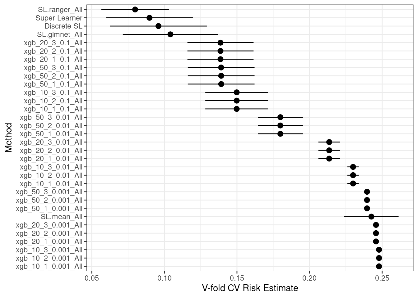
Finally, plot the performance for the different settings.

plot(cv_sl) + theme_bw()

Troubleshooting

If you get an error about predict for xgb.Booster, you probably need to install the latest version of XGBoost from github.

Citation

BibTeX citation:
@online{bochman2024,
  author = {Bochman, Oren},
  title = {SuperLearner},
  date = {2024-01-10},
  url = {https://orenbochman.github.io/posts/2024/2024-01-10-superlearner/},
  langid = {en}
}
For attribution, please cite this work as:
Bochman, Oren. 2024. “SuperLearner.” January 10, 2024. https://orenbochman.github.io/posts/2024/2024-01-10-superlearner/.