Scaling in financial prices: I. Tails and dependence
“The ideal market completely disregards those spikes—but a realistic model cannot.”
Mandelbrot highlights the inadequacy of models ignoring extreme price movements, emphasizing the need for a framework that can accommodate them.
In the paper “Scaling in financial prices: I. Tails and dependence” (Mandelbrot 2001) Mandelbrot surveys his research on modeling financial price fluctuations. Mandelbrot challenges the traditional Brownian motion model, arguing that financial data exhibits “fat tails” and long-range dependence, better captured by his multi-fractal model. He introduces the “star equation,” a mathematical framework expressing scaling invariance in financial prices. The paper presents graphical evidence supporting his claims and contrasts his models with traditional approaches, emphasizing the importance of considering both short-term and long-term data simultaneously. Finally, he discusses the implications for risk assessment and diversification strategies.
Paper Summary
Main Themes:
- Non-Gaussianity of financial price changes: Empirical evidence strongly suggests that price changes are not normally distributed, exhibiting “fat tails” with a higher frequency of extreme events than predicted by the standard Brownian motion model.
- Scaling and self-affinity: Financial price series exhibit similar patterns across different time scales, a concept mathematically described as self-affinity. This suggests the presence of underlying rules governing price variations across various time horizons.
- Limitations of traditional models: Models assuming independent and identically distributed price changes with finite variance, like the Brownian motion model, fail to capture the observed characteristics of financial data, particularly extreme price swings and volatility clustering.
- Multifractality as a potential solution: The concept of multifractality, which incorporates both long-range dependence and scale invariance, offers a promising framework for modeling financial price variations more realistically.
Most Important Ideas/Facts:
Empirical evidence of power laws: Studies reveal power-law distributions for both the tail probabilities of price changes (exponent α) and long-range dependence (exponent 2H-2).
- Fat tails: Mandelbrot’s early work (1963) showed evidence of power-law tails in cotton prices, later confirmed by Fama (1965) for a broader range of securities. These findings challenged the Gaussian assumption of price changes.
- Infinite dependence: The Hurst puzzle highlighted long-range dependence in price series, suggesting that price changes are not independent. Mandelbrot (1965) proposed a power law to describe this dependence.
Challenges to traditional scaling: Officer (1972) demonstrated deviations from scaling in financial data when applying the collapse test across different time increments, questioning the validity of models like Mandelbrot’s 1963 model based on Lévy stable distributions.
States of Variability and Randomness - Mandelbrot introduced this concept to categorize randomness into mild (Gaussian-like), slow (requiring adjustments for short-term behavior), and wild (exhibiting persistent non-Gaussianity across time scales). He argued that financial markets belong to the “wild” category.
Shortcomings of truncated power-law distributions: While some researchers have attempted to reconcile observed data with the Gaussian framework by truncating the tails of power-law distributions, this approach is criticized for being ad-hoc and destroying the scaling properties observed in financial markets.
The promise of multifractals: Mandelbrot proposed a model combining fractional Brownian motion and multifractal trading time to capture both long-range dependence and scale invariance in financial prices. This model has the potential to address the limitations of earlier models and provide a more accurate representation of financial market dynamics.
“I disagree that non-stationarity is obvious and do my best to avoid it.” 1{.aside}
1 This quote reflects Mandelbrot’s stance on the misleading emphasis on non-stationarity in financial data, advocating for the search for generalized forms of stationarity and corresponding models.
What are the key limitations of existing financial models?
Traditional models often assume that price changes are normally distributed, but empirical evidence suggests that this is not the case. [1] Financial prices tend to exhibit “fat tails,” meaning that extreme events are more common than a normal distribution would predict. [1, 2] This limitation is particularly important because models that fail to account for extreme price swings can be unreliable for risk management and other financial applications. [3]
Many financial models assume that price changes are independent and identically distributed, but this is also not supported by the data. [4, 5] Financial prices often exhibit long-range dependence, meaning that past price changes can influence future price changes. [5] Mandelbrot referred to this as the “Hurst puzzle.” [5]
Some researchers have tried to address these limitations by truncating the tails of power-law distributions, but this approach is problematic. [6] Truncating the tails can destroy the scaling properties observed in financial markets, leading to models that are not accurate. [6]
Mandelbrot argued that financial markets are “wildly variable” and that this variability cannot be ignored. [7] He suggested that models need to incorporate both long-range dependence and scale invariance to accurately capture financial market dynamics. [8]
Multifractal models offer a promising approach to address these limitations. [8-10] These models combine fractional Brownian motion and multifractal trading time to capture both long-range dependence and scale invariance in financial prices. [8] However, more research is needed to assess the effectiveness of multifractal models and to develop practical applications. [11, 12]
“Financial reality is not mildly variable even on the scale of a century. All things considered, one must adjust to the fact that financial reality is wildly variable. It would be totally unmanageable, unless there is some underlying property of invariance.”
This quote underscores the persistent non-Gaussianity of financial data and the crucial need for finding an invariance principle to model this “wild” behavior.
Next Steps:
- Further exploration of multifractal models: Delve deeper into the mathematical framework of multifractals and their application to financial markets.
- Empirical testing of multifractal models: Conduct rigorous statistical analysis to assess the effectiveness of multifractal models in capturing the observed properties of financial data.
- Developing practical applications: Explore the potential of multifractal models for risk management, portfolio optimization, and other practical applications in finance.
Q&A
What is the main challenge in representing financial price variation through mathematical models?
The main challenge lies in capturing the complex and seemingly erratic behavior of financial prices over different time scales. Traditional models like Brownian motion struggle to accurately represent the large price fluctuations (“spikes”), periods of high volatility clustering, and long-term dependencies observed in real market data.
How does the concept of “scaling” address this challenge?
Scaling, in the context of financial markets, postulates that price patterns exhibit similar statistical properties across various time scales. This concept implies the existence of underlying rules governing price fluctuations, even if those rules may appear complex.
What are the limitations of traditional models like Brownian motion in capturing the behavior of financial prices?
Brownian motion assumes independent and normally distributed price changes. This assumption fails to account for the “fat tails” observed in actual price distributions, which indicate a higher probability of extreme events than predicted by a normal distribution. Additionally, Brownian motion does not address the clustering of volatility and long-range dependencies evident in real markets.
What is the significance of the “Officer effect”?
The Officer effect refers to empirical observations demonstrating that the simple scaling properties assumed in early models like Mandelbrot’s 1963 model do not hold consistently across different time increments for various financial assets. This finding highlighted the need for more sophisticated models to capture the complexities of market behavior.
What is meant by “states of variability and randomness” and how does this concept relate to financial modeling?
Mandelbrot proposed three states of variability and randomness: mild, slow, and wild. Mild randomness resembles the behavior of a gas, characterized by independent events and normal distributions, as exemplified by Brownian motion. Slow randomness, analogous to liquids, introduces some degree of dependence or “memory” in the system. Wild randomness, similar to solids, exhibits strong dependencies and large fluctuations, reflecting the reality of financial markets. Understanding these states is crucial for developing appropriate models and managing risk.
What are the key features of Mandelbrot’s multifractal model for asset returns?
Mandelbrot’s multifractal model combines fractional Brownian motion (FBM) and multifractal trading time (MTT). This compound process allows for long-range dependence and captures the observed volatility clustering and fat tails in price distributions. Unlike earlier models, the multifractal model acknowledges the inherent “wild” randomness of financial markets.
How does the multifractal model address the limitations of previous models and account for empirical observations like the Officer effect?
By incorporating both FBM and MTT, the multifractal model accounts for the long-term dependencies and varying volatility observed in financial time series. This approach allows for a more accurate representation of price fluctuations over a wide range of time scales, thereby addressing the shortcomings of previous models that relied on assumptions of independence and normal distributions.
What are the implications of the multifractal model for understanding and managing risk in financial markets?
The multifractal model highlights the presence of “wild” randomness in financial markets, implying that traditional risk management techniques based on normal distributions and independence assumptions may be inadequate. This model emphasizes the importance of considering the possibility of extreme events and the clustering of volatility when assessing and managing risk.
A Study Guide
Quiz
Instructions: Answer the following questions in 2-3 sentences each.
What is the key question regarding the power-law distribution of financial price changes, and how does it relate to the concepts of independent increments and the multifractal model?
The key question is whether the exponent α in the power-law distribution is restricted to α < 2, which is the case for independent increments as in the Lévy-stable model. The multifractal model allows for dependent increments and α > 2.
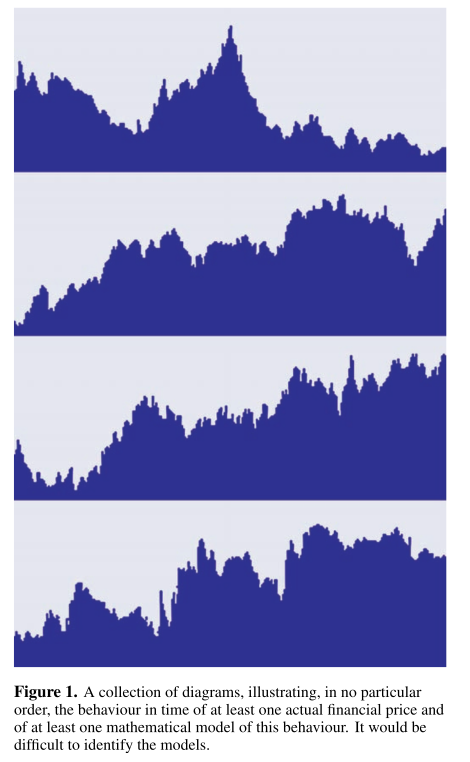
- What is the visual challenge presented by Figure 1, and why is it misleading to conclude that Brownian motion adequately represents actual price data based on this figure?
Figure 1, showing price levels, makes different models and real data visually indistinguishable. It’s misleading to conclude Brownian motion is adequate because it only shows overall trends and hides crucial details about price change behavior.
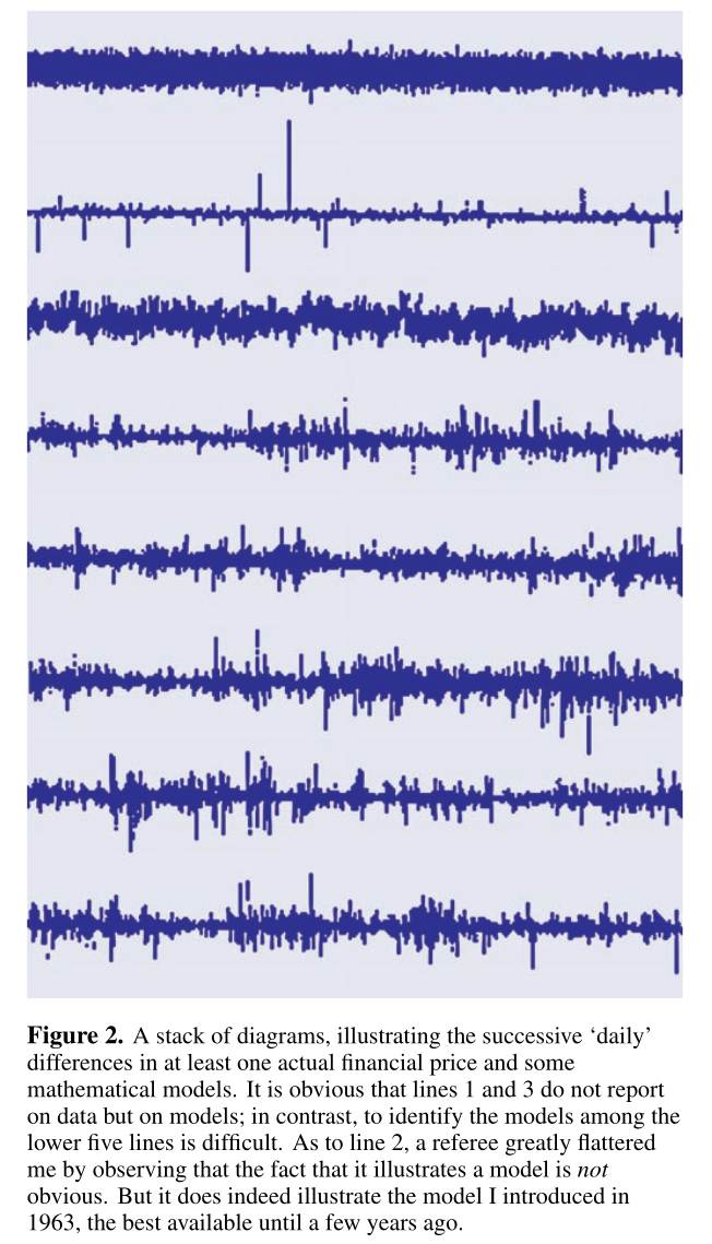
How does Figure 2 provide a clearer picture of price changes compared to Figure 1, and what key characteristics of real market data does it reveal?
Figure 2 plots daily price increments, highlighting significant differences between models and real data. It reveals key characteristics like spikes (large price changes), varying strip width (volatility) and spike clustering, absent in Brownian motion.
- Why is the ideal market hypothesis inadequate in capturing the true nature of financial markets, particularly concerning extreme price changes?
The ideal market hypothesis fails to account for extreme price changes (“spikes”), which are statistically improbable in a Gaussian framework but common in real markets. These events, though infrequent, contribute disproportionately to overall market behavior.
What is the author’s perspective on the relationship between short- and long-term price variations, and how does this differ from the conventional approach?
The author argues that price variations exhibit similar characteristics across different time scales, suggesting common underlying rules. This contrasts with the conventional view of separate models for different time horizons.
Explain the concept of self-affinity and its significance in representing market behavior.
Self-affinity is a scaling property where a shape’s parts are scaled versions of the whole, but with different scaling factors for different dimensions. In market charts, this reflects the similarity of patterns at different time scales, albeit with adjusted price scales.
Describe the three special cases of the compound process BH[θ(t)] and how they relate to earlier financial models.
The special cases are:
- Bachelier model: H=1/2, θ(t)=t, resulting in standard Brownian motion;
- M1965 model: H≠1/2, θ(t)=t, yielding fractional Brownian motion;
- M1963 model: H=1/2, θ(t) is a stable subordinator, leading to a Lévy-stable process.
What is the key difference between subordination and general compounding in the context of the FBM (MTT) model, and what advantage does general compounding offer?
Subordination uses only monotone, non-decreasing processes for θ(t), preserving independent increments. General compounding allows for dependent increments in θ(t), enabling the FBM(MTT) model to capture more complex and realistic price dynamics.
How does the concept of ‘states of variability and randomness’ contribute to understanding the varying effectiveness of risk reduction through diversification?
Different ‘states of variability and randomness’ (mild, wild, slow) impact the effectiveness of risk reduction. Mild randomness allows for efficient averaging (e.g., diversification), while wild randomness, characterizing financial markets, can hinder or nullify this effect.
Why does the author consider the search for transients towards Brownian motion a “thoroughly ill-conceived idea,” and what alternative approach does he propose?
The author argues that deviations from Brownian motion persist even at very large time scales, indicating that financial markets are inherently ‘wildly variable’.
Instead of searching for convergence to the Brownian, he proposes seeking invariant properties within this ‘wildness’, leading to the multifractal model.
Essay Questions
- Discuss the limitations of the traditional financial models based on Brownian motion and Gaussian distributions. How do these models fail to capture the empirical realities of financial markets, particularly in terms of extreme price changes and long-range dependence?
- Explain the concept of scaling and its role in the development of Mandelbrot’s models of financial price variation. Compare and contrast the scaling properties of the M1963, M1965, and M1972/1997 models.
- Elaborate on the concept of multifractal trading time (MTT) and its significance in the M1972/1997 model. How does incorporating MTT allow for a more realistic representation of market volatility and price fluctuations?
- Analyze the implications of the “Officer effect” for financial modeling. How did this empirical observation challenge the prevailing assumptions about scaling and lead to the development of more sophisticated approaches?
- Discuss the concept of “states of variability and randomness” and its relevance to understanding risk and diversification in financial markets. How do the characteristics of “wild randomness” in financial data affect the effectiveness of traditional risk management techniques?
Glossary of Key Terms
- Power-law distribution
- A probability distribution where the tail probabilities decay as a power of the variable. In financial markets, this refers to the distribution of price changes.
- Independent increments
- A property of stochastic processes where increments over non-overlapping time intervals are statistically independent.
- Multifractal model
- A model of asset returns that incorporates both long-range dependence and fat tails in the distribution of price changes.
- Brownian motion
- A continuous-time stochastic process where increments are independent and normally distributed. Volatility: A measure of the dispersion of price changes over time.
- Self-affinity
- A scaling property where parts of a shape are scaled versions of the whole, but with different scaling factors for different dimensions.
- Fractional Brownian motion (FBM)
- A generalization of Brownian motion that allows for long-range dependence.
- Multifractal trading time (MTT)
- A non-linear transformation of clock time that accounts for the changing volatility in financial markets.
- Subordination
- A method of constructing a new stochastic process by replacing the time variable of an existing process with a new, independent process.
- General compounding
- A more general method of combining two stochastic processes, allowing for dependence between the processes.
- States of variability and randomness
- A categorization of randomness into mild, wild, and slow, reflecting the degree of structure and variability.
- Officer effect
- Empirical observation that the scaling properties of financial price changes vary with the time increment used to measure the changes.
- Critical moment exponent
- A parameter α that determines the highest moment of a distribution that is finite.
Citation
@online{bochman2024,
  author = {Bochman, Oren},
  title = {Scaling in Financial Prices 1},
  date = {2024-11-28},
  url = {https://orenbochman.github.io/posts/2024/2024-11-28-misbahaviour-of-markets/part1/},
  langid = {en}
}


