Roth Erev learning in Lewis signaling games

Learning in Lewis signaling games

I wish now to implement learning in the Lewis signaling game. In the book some reinforcement learning RL algorithms are presented in some detail and a few variations are mentioned. It worthwhile pointing out that the book statement of the algorithms is good enough to understand how the algorithms operate in general. However some of the details required to implement the algorithms were glossed over. As my one time collage Yuri Stool like to point out, “the devil is in the details.”

I ended up implementing the algorithms a number of times - once to get it to work, second time to develop my own algorithm as I gained new insights into the problems. A third time after reading more of the papers whihc suggested how more details on conducting experiments which led to a deeper understanding of enumerating and ranking the partial pooling equilibria. The point here is that natural language is mostly a separating equilibrium - most words are unambiguous but there are a significant subset of words that have multiple meaning and there are many synonyms. Mechanisms in the lexicon seem to eventually resolves some ambiguities while letting others persist indefinitely. So while the separating equilibria are of primary interests in reality users if signaling systems satisfice with a systems that is good enough. This are the much more common partial pooling variants with high degree of separation plus a context based disambiguation mechanism. I consider the erosion of English and Latin conjugation and declination after the classical period as a simpler contextual disambiguation mechanism dismantling a nearly perfect signaling subsystem with a rather degenerate one with high degree of partial pooling. A simulation might show how a few prepositions and auxilary verbs are more efficent to learn and process than fully inflected systems of case and verb ending (especially if modified by phonetics). But my guess is that this happened as more speakers had to master an use a core language, without access to resources for learning the classical forms. I guess the dark ages and a decline in literacy likely speed up the process.

Adding better analysis, estimating expected returns for a set of weights, tracking regret during learning. Considering different path to salience via differntial risks/costs for signals, and non uniform state distribution.

The big question seems to be:

What is a simple rl algorithm to evolve and disseminate a signaling system with certain added requirements like

complex signals
- conjunctive signal aggregation
- ordered signal aggregation via learning a grammar like SVO.
- recursive signal aggregation replacing linear ordered with a partial order.
resolving ambiguity by context
mechanism for correcting errors (vowel harmony, agreement)
simple growth of the lexicon (black bead leads to mutation in the urn model)
sufficient capacity,
minimal burden for processing (extending inference mechanism to reduce cognitive load, compress messages, erode unneeded structures)
minimal burden in learning (e.g. by generalization via regularity in morphology, and syntax)
high accuracy for transmission of messages
saliencey - a information theoretic measure of more efficient transition subset of states/messages pairs.

Where the great unknown seems to be to find a minimal extension to the Lewis game in which all these might evlove.

Having stated the problem in detail lets me make the following two observations:

The aggregation rules for complex signaling should be made to arise by imposing costs on systems under which agents more frequently fail to make good inference with high probability of a partials message’s describing risky states for sender and or receiver.
A second cost to fitness is the role of mistakes in signaling and or receiving. (ie. adding an small chance for decoding similar sounding signals (homophones, short vs long sounds, hissed and hushed, round, front and back vouwels). This may lead to excluding simple signals from places they might be confused, is it (a,a) (a.a) or (aa,a), (a,_,a) are avoided if signal ‘a’ is excluded from the first positions (say verb class). here dot might be a short pause, comma a long pause, undescore an unmarked slot, and two aa no pause. (either two a or a long a.) if we prefix V with v S with s and P with C

we end up with a system that is much more robust. And we may have the added bonus that we can easily detect a tree formation based on multiple Vprefix in the sentence….
1. word grammar
2. sub word grammar - a complex morphology - highly regular yet differented complex signals
3. this could lead to redundancy based Error correction like subject verb agreement, noun adjective agreement or vowel harmony.
4. Concord - case agreement (nouns pronouns and adjective are in agreement)
Ease of processing
1. agreement can also ease processing
2. assimilation and elision
3. limiting processing/disabihation context windows.
4. word order
5. however redundencies add overhead, making signals longer and may make learning much longer (this is when we students who generelize are wrong and then need to learn via negative examples.
If many we have different complex signaling systems with minimal mistakes are possible one would prefer a system that is easier to learn. (Shorter lexicon, with lower chances of collision. Shorter grammar, fewer negtive examples, more room for expansion)

Richard Herrnstein’s Matching law

we start with some initial weights, perhaps equal.
An act is chosen with probability proportional to its weight.
The payoff gained is added to the weight for the act that was chosen,
and the process repeats

Roth-Erev learning algorithm

set starting weight for each option
weights evolve by addition of rewards gotten
probability of choosing an alternative is proportional to its weight.

Bush-Mosteller learning

set starting weight for each option
weights evolve by addition of rewards gotten
probability of choosing an alternative is proportional to its weight.
if the reward is 0 the weight is multiplied by a forgetting factor.

Roth-Erev learning with forgetting:

set starting weight for each option
weights evolve by addition of rewards gotten
probability of choosing an alternative is proportional to its weight.
if the reward is 0 the weight is multiplied by a forgetting factor.

ARP learning

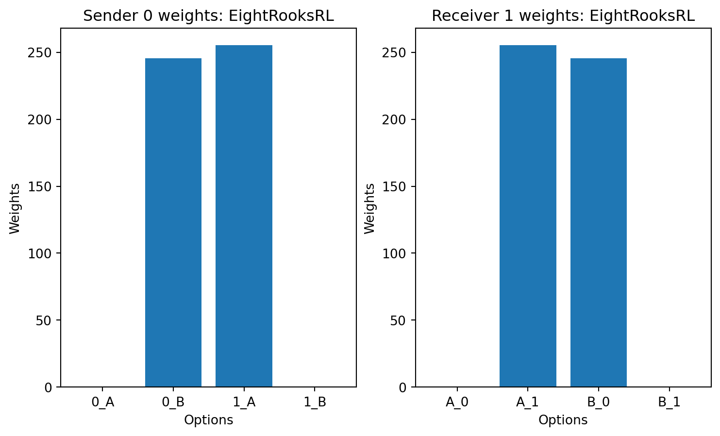
Bochman 8-Rooks RL

this is a special purpose rl algorithm for coordination problems where agents need to establish a convention like in the Lewis signaling game. The idea is that the matrix is similar to a placing 8 rooks on on a chess board with no two under attack. In this case once an option has been chosen we want to exclude all options that shares a row or a collumm. So we set to zero any weights which share the same prefix or suffix as a reward 1 option.

set starting weight for each option (state_signal) for the sender and (signal_action) for the receiver, perhaps to 1
weights evolve by

addition of rewards gotten for a correct choice and
zeroing of options with the same prefix or suffix to exclude them from the choice set.

probability of choosing an alternative is proportional to its weight.

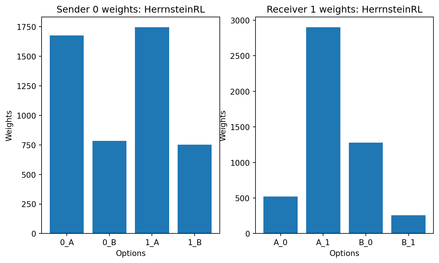
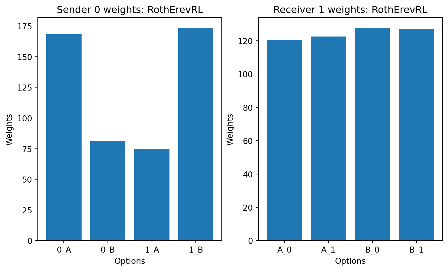
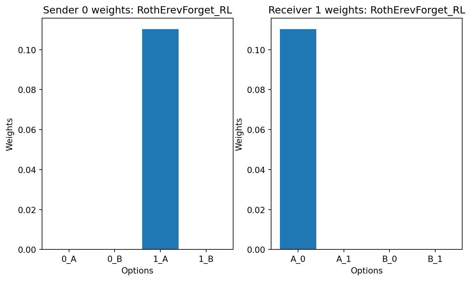
from mesa import Agent, Model
from mesa.time import StagedActivation
import random
import numpy as np
import matplotlib.pyplot as plt
from abc import ABC, abstractmethod

# let's define a lambda to take a list of options and intilize the weights uniformly 
uniform_init = lambda options, w : {option: w for option in options}
random_init  = lambda options, w : {option: random.uniform(0,1) for option in options}

# lets make LeaningRule an abstract class with all the methods that are common to all learning rules
# then we can subclass it to implement the specific learning rules
class LearningRule(ABC):
  
    def __init__(self, options, learning_rate=0.1,verbose=False,name='LearningRule',init_weight=uniform_init):
        self.verbose = verbose
        self.name=name
        self.learning_rate = learning_rate
        if self.verbose:
          print(f'LearningRule.__init__(Options: {options})')
        self.options = options
        self.weights = init_weight(options,1.0) # Start with one ball per option 
        
        
    def get_filtered_weights(self, filter):
        if self.verbose:
          print(f'get_filtered_weights({filter=})')
        # if filter is int convert to string
        if isinstance(filter, int):
            filter = str(filter)
        filter_keys = [k for k in self.weights.keys() if k.startswith(filter)]
        weights = {opt: self.weights[opt] for opt in filter_keys}
        return weights
      
    @abstractmethod
    def choose_option(self,filter):
        pass
      
    @abstractmethod
    def update_weights(self, option, reward):
        pass
      
class HerrnsteinRL(LearningRule):
    '''
                                    The Urn model
     nature            sender                 reciever     reward
                       
    | (0) | --{0}-->  | (0_a)  | --{a}--> | (a_0) | --{0}-->   1   
    |     |           | (0_b)  | --{b}    | (a_1) | --{1}-->   0
    |     |           +--------+    | +-->+-------+
    |     |                         +-|-+  
    | (1) | --{1}-->  | (1_a)  | --{a}+ +>| (b_0) | --{1}-->   1
    |     |           | (1_b)  | --{b}--->| (b_1) | --{0}-->   0
    +-----+           +--------+          +-------+
    
    
    Herrnstein urn algorithm
    ------------------------
    
    1. nature picks a state 
    2. sender  gets the state, chooses a signal by picking a ball in choose_option() from the stat'es urn
    3. reciver gets the action, chooses an actuion by picking a ball in choose_option()
    4. the balls in the urns are incremented if action == state
    5. repeat
    
    '''
    def __init__(self, options, learning_rate=1.0,verbose=False,name='Herrnstein matching law'):
      
        super().__init__(verbose = verbose, options=options, learning_rate=learning_rate,name=name)

    def update_weights(self, option, reward):
      
        old_weight = self.weights[option]
        self.weights[option] += self.learning_rate * reward 
        if self.verbose:
          print(f"Updated weight for option {option}: {old_weight} -> {self.weights[option]}")
          
    def choose_option(self,filter):
      
        '''
        
        '''
        # subseting the weights by the filter simulates different urns per state or signal
        weights = self.get_filtered_weights(filter)

        # calculate their probabilities then
        total = sum(weights.values())
        assert total > 0.0, f"total weights is {total=} after {filter=} on {self.weights} "
        probabilities = [weights[opt] / total for opt in weights]
        # then drawn an option from the filtered option using the probabilities
        return np.random.choice(list(weights.keys()), p=probabilities)


class RothErevRL(LearningRule):

    def __init__(self, options, learning_rate=0.1,verbose=False,name='Roth Erev RL'):
      
        super().__init__(verbose = verbose, options=options, learning_rate=learning_rate,name=name)

    def update_weights(self, option, reward):
        old_weight = self.weights[option]
        if reward == 1:
          self.weights[option] += self.learning_rate * reward
        if self.verbose:
          print(f"Updated weight for option {option}: {old_weight} -> {self.weights[option]}")

    def choose_option(self,filter):
        # we subset the weights by the filter, calculate their probabilities then
        # then drawn an option from the filtered option using the probabilities
        weights = self.get_filtered_weights(filter)
        total = sum(weights.values())
        probabilities = [weights[opt] / total for opt in weights]
        return np.random.choice(list(weights.keys()), p=probabilities)
  

class RothErevForget_RL(LearningRule):

    def __init__(self, options, learning_rate=0.1,verbose=False,name='Roth Erev with forgetting'):
      
        super().__init__(verbose = verbose, options=options, learning_rate=learning_rate,name=name)

    def update_weights(self, option, reward):
        old_weight = self.weights[option]
        if reward == 1:
          self.weights[option] += self.learning_rate * reward
        else:
          self.weights[option] *= self.learning_rate 
        if self.verbose:
          print(f"Updated weight for option {option}: {old_weight} -> {self.weights[option]}")

    def choose_option(self,filter):
        weights = self.get_filtered_weights(filter)
        total = sum(weights.values())
        probabilities = [weights[opt] / total for opt in weights]
        return np.random.choice(list(weights.keys()), p=probabilities)
  
class EightRooksRL(LearningRule):
    def __init__(self, options, learning_rate=0.1,verbose=False,name='Eight Rooks RL'):
        super().__init__(verbose = verbose, options=options, learning_rate=learning_rate,name=name)


    def update_weights(self, option, reward):
        self.prefix = option.split('_')[0]
        self.suffix = option.split('_')[1]
        
        old_weights=self.weights.copy()
        
        for test_option in self.options:
          if reward == 1:
            if test_option == option:
            # increment the weight of the good option 
              self.weights[test_option] += self.learning_rate * reward
            elif test_option.startswith(self.prefix) or test_option.endswith(self.suffix) :
            # decrement all other options with same prefix  or suffix
               # if self.weights[test_option] < 0.000001:
               #   self.weights[test_option] = 0.0
               # else:
                self.weights[test_option] *= self.learning_rate 
          # elif test_option == option:
          #   # decrement the weights of the bad option combo
          #   self.weights[option] *= self.learning_rate 

        if self.verbose:
          print()
          for option in self.options:
            if old_weights[option] != self.weights[option]:
              print(f"{option}: weight {old_weights[option]} -> {self.weights[option]}")
          #print(f"Updated weight {old_weights} -> {self.weights}")


    def choose_option(self,filter):
        weights = self.get_filtered_weights(filter)
        total = sum(weights.values())
        probabilities = [weights[opt] / total for opt in weights]
        # if there is a max weight return it otherwise return a random option from the max wights
        if len([opt for opt in weights if weights[opt]==max(weights.values())]) == 1:
          return max(weights, key=weights.get)
        else:
          return np.random.choice([opt for opt in weights if weights[opt]==max(weights.values())])

class LewisAgent(Agent):
    def __init__(self, unique_id, model, learning_options, learning_rule, verbose=False):
        super().__init__(unique_id, model)
        self.message = None
        self.action = None
        self.reward = 0
        self.learning_rule = learning_rule
        self.verbose = verbose
        
    def send(self):
      return
    
    def receive(self):
      return
    
    def calc_reward(self):
      return

    def set_reward(self):
        self.reward = self.model.reward
        if self.verbose:
          print(f"Agent {self.unique_id} received reward: {self.reward}")
        
    def update_learning(self):
        self.learning_rule.update_weights(self.option, self.reward)  # Update weights based on signals and rewards        

class Sender(LewisAgent):
    def send(self):
        state = self.model.get_state()
        #self.message = self.learning_rule.choose_option(filter=state)  # Send a signal based on the learned weights
        
        self.option = self.learning_rule.choose_option(filter=state)  # Send a signal based on the learned weights
        self.message = self.option.split('_')[1]
        if self.verbose:
          print(f"Sender {self.unique_id} sends signal for state {state}: {self.message}")

class Receiver(LewisAgent):
    def receive(self):
        self.received_signals = [sender.message for sender in self.model.senders]  # Receive signals from all senders
        #print(f"Receiver {self.unique_id} receives signals: {self.received_signals}")
        if self.received_signals:
            for signal in self.received_signals:
                self.option = self.learning_rule.choose_option(filter=signal)  # Choose an action based on received signals and learned weights
                self.action = int(self.option.split('_')[1])
                if self.verbose:
                  print(f"Receiver {self.unique_id} receives signals: {self.received_signals} and chooses action: {self.action}")


    def calc_reward(self):
        correct_action = self.model.current_state
        self.model.reward = 1 if self.action == correct_action else 0
        if self.verbose:
          print(f"Receiver {self.unique_id} calculated reward: {self.reward} for action {self.action}")

class SignalingGame(Model):
    def __init__(self, 
                senders_count=1, 
                receivers_count=1, k=3,
                learning_rule=LearningRule,
                learning_rate=0.1,
                verbose=False):
        super().__init__()
        self.verbose = verbose
        self.k = k
        self.current_state = None
        self.learning_rate=learning_rate

        # Initialize the states, signals, and actions mapping
        self.states = list(range(k))  # States are simply numbers
        self.signals = list(chr(65 + i) for i in range(k))  # Signals are characters
        self.actions = list(range(k))  # Actions are simply numbers

        # generate a list of state_signal keys for the sender's weights
        self.states_signals_keys = [f'{state}_{signal}' for state in self.states for signal in self.signals]
        # generate a list of signal_action keys for the receiver's weights
        self.signals_actions_keys = [f'{signal}_{action}' for signal in self.signals for action in self.actions]
        
        self.senders = [Sender(i, self, learning_options=self.states_signals_keys, 
                                  learning_rule=learning_rule(self.states_signals_keys, self.learning_rate,verbose=self.verbose)
                              ) for i in range(senders_count)]
        self.receivers = [Receiver(i + senders_count, self, learning_options=self.signals_actions_keys, 
                                  learning_rule=learning_rule(self.signals_actions_keys, self.learning_rate,verbose=self.verbose)
                              ) for i in range(receivers_count)]
        
        self.schedule = StagedActivation(self, 
          agents = self.senders + self.receivers, 
          stage_list=['send', 'receive', 'calc_reward', 'set_reward', 'update_learning'])

    def get_state(self):
        return random.choice(self.states)

    def step(self):
        self.current_state = self.get_state()
        if self.verbose:
          print(f"Current state of the world: {self.current_state}")
        self.schedule.step()


# function to plot agent weights side by side

def plot_weights(sender,reciver,title='Agent'):
    fig, ax = plt.subplots(1,2,figsize=(9,5))
    weights = sender.learning_rule.weights
    ax[0].bar(weights.keys(), weights.values())
    ax[0].set_xlabel('Options')
    ax[0].set_ylabel('Weights')
    ax[0].set_title(f'Sender {sender.unique_id} weights: {title}')
    
    weights = reciver.learning_rule.weights
    ax[1].bar(weights.keys(), weights.values())
    ax[1].set_xlabel('Options')
    ax[1].set_ylabel('Weights')
    ax[1].set_title(f'Receiver {reciver.unique_id} weights: {title}')
    plt.show()


# Running the model
k=2
verbose = False
for LR in [HerrnsteinRL,
           RothErevRL,
           RothErevForget_RL,
           EightRooksRL
           ]:
  print(f"--- {LR.__name__} ---")
  if LR == HerrnsteinRL:
    learning_rate=1.
  else:
    learning_rate=.1
  model = SignalingGame(senders_count=1, receivers_count=1, k=k, learning_rule=LR,learning_rate=learning_rate,verbose=verbose)
  for i in range(10000):
      if verbose:
        print(f"--- Step {i+1} ---")
      model.step()
      # 
      #print the agent weights
  #print('Sender weights:',model.senders[0].learning_rule.weights)
  # plot weights side by side
  
  plot_weights(model.senders[0],model.receivers[0],title=LR.__name__)
  #print('Receiver weights:',model.receivers[0].learning_rule.weights)
  #plot_weights(model.receivers[0],title=LR.__name__)

--- HerrnsteinRL ---
--- RothErevRL ---
--- RothErevForget_RL ---
--- EightRooksRL ---

/home/oren/work/blog/env/lib/python3.10/site-packages/mesa/time.py:82: FutureWarning:

The AgentSet is experimental. It may be changed or removed in any and all future releases, including patch releases.
We would love to hear what you think about this new feature. If you have any thoughts, share them with us here: https://github.com/projectmesa/mesa/discussions/1919

currently only the eight rooks learning rule is producing consistently good signaling systems. The other learning rules are not learning to signal correctly.

Please suggest how to fix this - according to the literature the Roth-Erev with forgetting learning rule should work well in this case.

TODO: implement Bush-Mosteller learning - as this is a match for population dynamics.

TODO: also implement population dynamics as it may not be clear that BM RL is a perfect fit for population dynamics under all lewis game conditions.

TODO: implement ARP learning.

TODO: implement epsilon-greedy, UCB and thompson sampling urn schemes, and Contextual bandits associative search (that’s our multiurn bandit)

Estimating the Gittins index for a Lewis games.

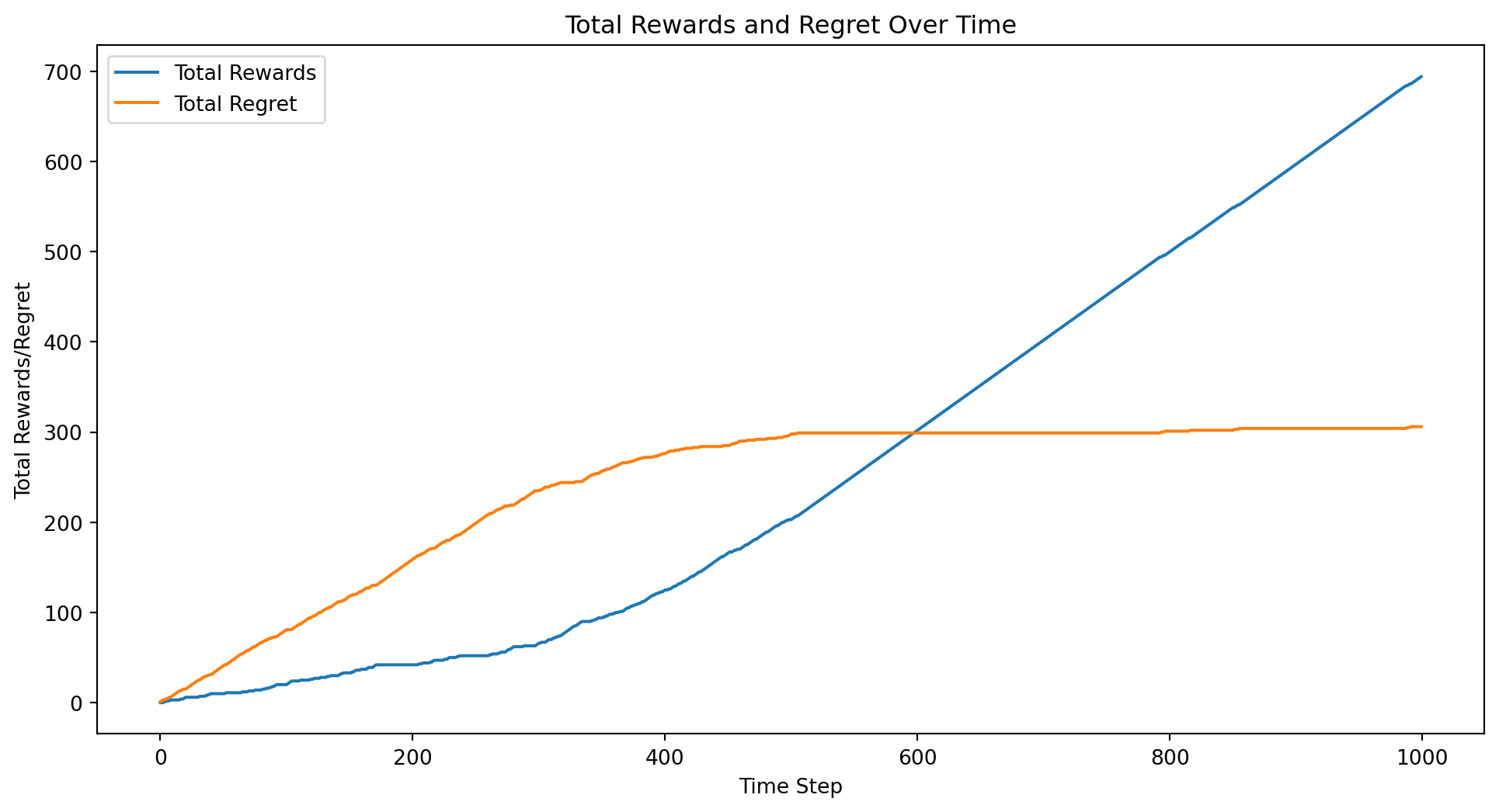
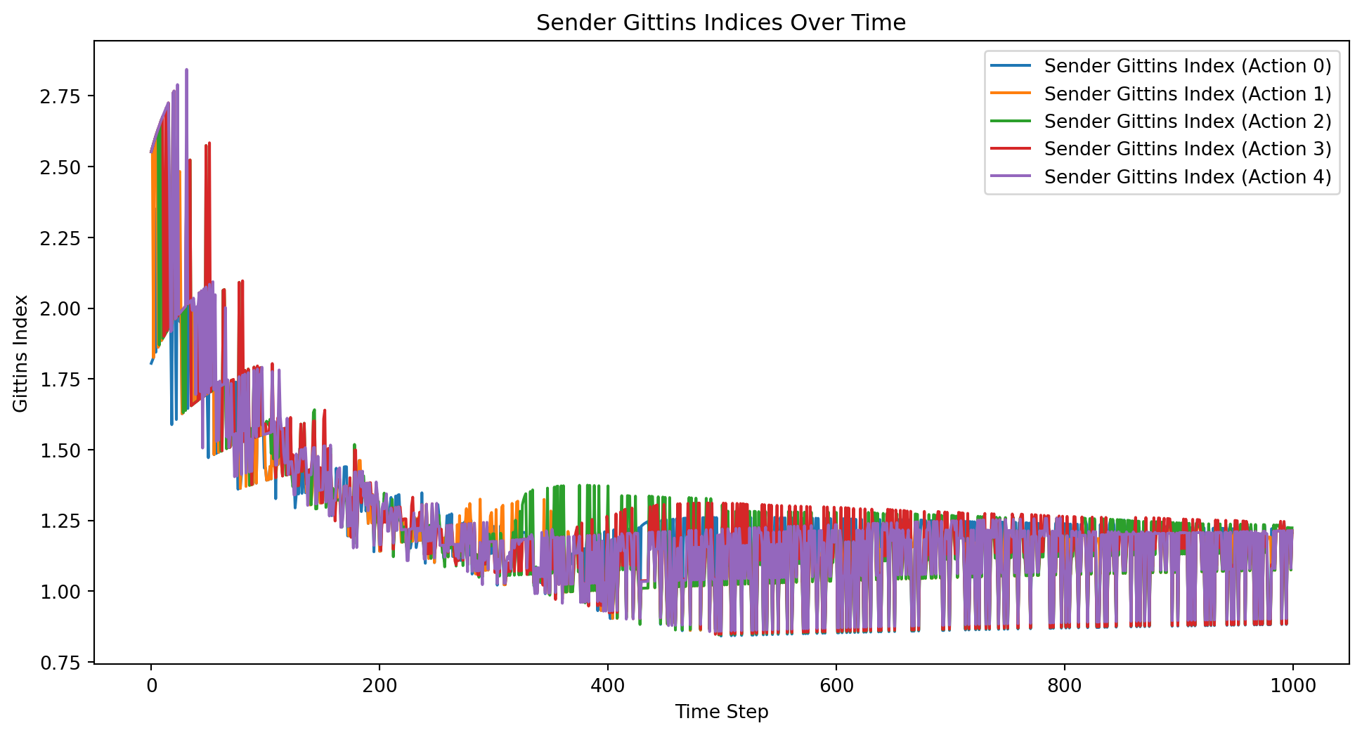
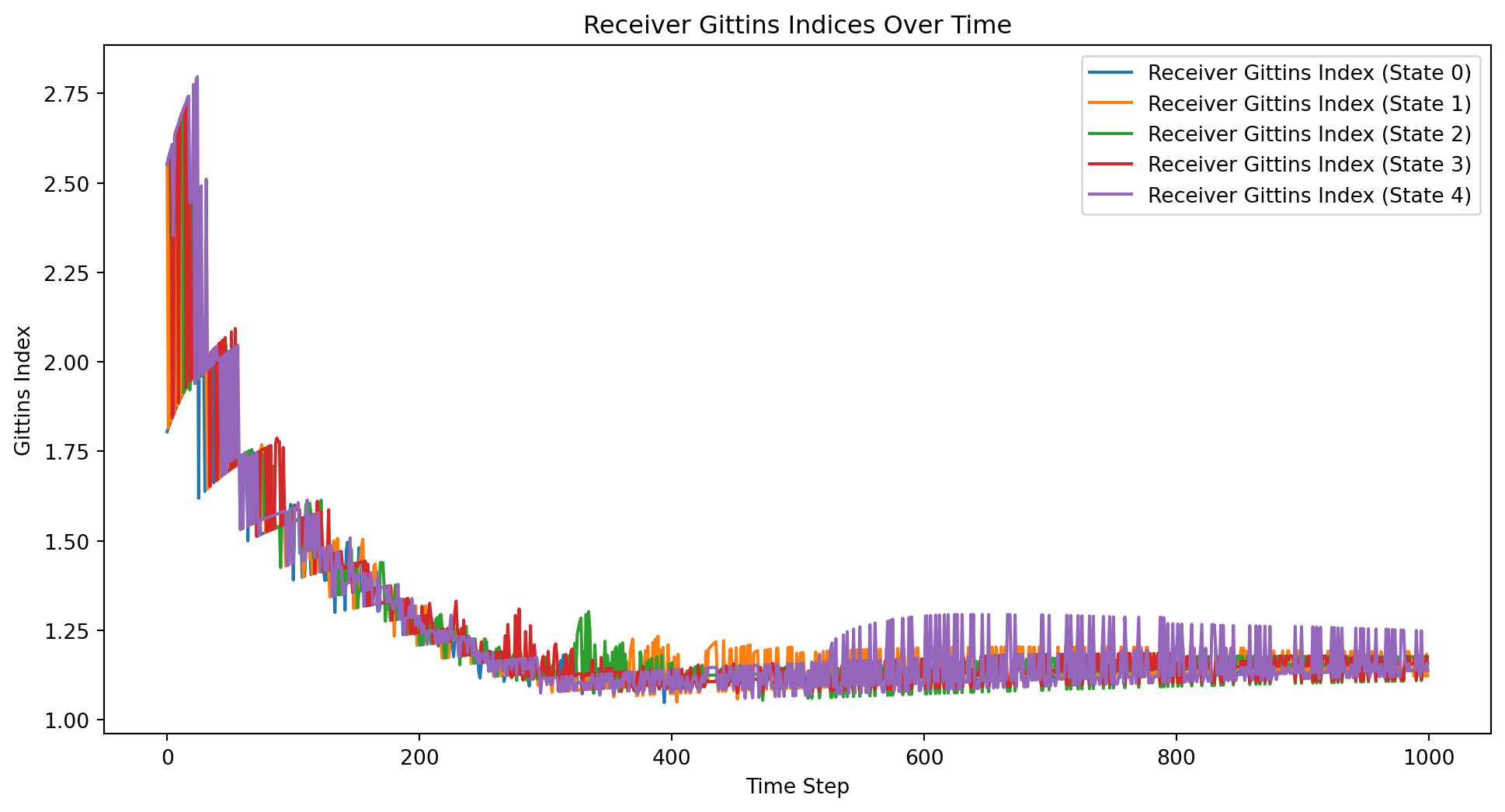
import numpy as np
import matplotlib.pyplot as plt

class ContextualBandit:
    def __init__(self, n_states, n_actions):
        self.n_states = n_states
        self.n_actions = n_actions
        self.rewards = np.zeros((n_states, n_actions))
        self.counts = np.ones((n_states, n_actions))

    def update(self, state, action, reward):
        self.counts[state, action] += 1
        self.rewards[state, action] += reward

    def get_gittins_index(self, state, action):
        # Simplified Gittins index computation
        total_reward = self.rewards[state, action]
        total_count = self.counts[state, action]
        return total_reward / total_count + np.sqrt(2 * np.log(np.sum(self.counts)) / total_count)

    def select_action(self, state):
        gittins_indices = [self.get_gittins_index(state, a) for a in range(self.n_actions)]
        return np.argmax(gittins_indices)

def sample_state(distribution, n_states):
    if distribution == "uniform":
        return np.random.randint(n_states)
    elif distribution == "normal":
        state = int(np.random.normal(loc=n_states/2, scale=n_states/6))
        return np.clip(state, 0, n_states - 1)
    else:
        raise ValueError("Unsupported distribution type")


# Example usage
n_states = 5
n_actions = 5
n_iterations = 1000

sender_bandit = ContextualBandit(n_states, n_actions)
receiver_bandit = ContextualBandit(n_actions, n_states)
state_distribution = "uniform"  # Change to "normal" for normal distribution

rewards = []
regrets = []
total_reward = 0
total_regret = 0
sender_gittins_indices = [[] for _ in range(n_actions)]
receiver_gittins_indices = [[] for _ in range(n_states)]

# Simulate the learning process
for t in range(n_iterations):
    state = sample_state(state_distribution, n_states)
    sender_action = sender_bandit.select_action(state)
    receiver_action = receiver_bandit.select_action(sender_action)
    
    reward = 1 if receiver_action == state else 0
    total_reward += reward
    total_regret += 1 - reward
    
    rewards.append(total_reward)
    regrets.append(total_regret)
    
    sender_bandit.update(state, sender_action, reward)
    receiver_bandit.update(sender_action, receiver_action, reward)
    
    for action in range(n_actions):
        sender_gittins_indices[action].append(sender_bandit.get_gittins_index(state, action))
    
    for state in range(n_states):
        receiver_gittins_indices[state].append(receiver_bandit.get_gittins_index(sender_action, state))

# Print final policy
print("Sender policy:")
for state in range(n_states):
    print(f"State {state}: Action {sender_bandit.select_action(state)}")

print("Receiver policy:")
for action in range(n_actions):
    print(f"Action {action}: State {receiver_bandit.select_action(action)}")

# Plot the total rewards and regrets over time
plt.figure(figsize=(12, 6))
plt.plot(rewards, label='Total Rewards')
plt.plot(regrets, label='Total Regret')
plt.xlabel('Time Step')
plt.ylabel('Total Rewards/Regret')
plt.title('Total Rewards and Regret Over Time')
plt.legend()
plt.show()

# Plot the Gittins indices over time for the sender
plt.figure(figsize=(12, 6))
for action in range(n_actions):
    plt.plot(sender_gittins_indices[action], label=f'Sender Gittins Index (Action {action})')
plt.xlabel('Time Step')
plt.ylabel('Gittins Index')
plt.title('Sender Gittins Indices Over Time')
plt.legend()
plt.show()

# Plot the Gittins indices over time for the receiver
plt.figure(figsize=(12, 6))
for state in range(n_states):
    plt.plot(receiver_gittins_indices[state], label=f'Receiver Gittins Index (State {state})')
plt.xlabel('Time Step')
plt.ylabel('Gittins Index')
plt.title('Receiver Gittins Indices Over Time')
plt.legend()
plt.show()

Sender policy:
State 0: Action 4
State 1: Action 0
State 2: Action 2
State 3: Action 3
State 4: Action 1
Receiver policy:
Action 0: State 1
Action 1: State 4
Action 2: State 2
Action 3: State 3
Action 4: State 0

Making it Bayesian

According to (Sutton and Barto 2018) Gitting’s index are usually associated with the Bayesian paradigm.

Sutton, R. S., and A. G. Barto. 2018. Reinforcement Learning, Second Edition: An Introduction. Adaptive Computation and Machine Learning Series. MIT Press. http://incompleteideas.net/book/RLbook2020.pdf.

As such one should be able to we could use a Bayesian updating scheme to learn expected rewards based on success counts. Since we are tracking successes vs failures we can use beta-binomial conjugate distributions to keep track of successes, failures and their likelihood.

This most basic form is like so:

Table 1: sender & receiver prior

(a) sender alpha, beta

State/Signal	0	1	2
0	0,0	0,0	0,0
1	0,0	0,0	0,0
2	0,0	0,0	0,0

(b) receiver alpha, beta

Signal/Action	0	1	2
0	0,0	0,0	0,0
1	0,0	0,0	0,0
2	0,0	0,0	0,0

Where we have a table of independent beta-binomial priors for each state/signal and signal/action pair.

After 5 failures we update the beta distribution for the sender and receiver as follows:

Table 2: sender alpha, beta

State/Signal	0	1	2
0	0,1	0,2	0,0
1	0,0	0,1	0,0
2	0,0	0,0	0,1

Table 3: receiver alpha, beta

Signal/Action	0	1	2
0	0,1	0,0	0,1
1	0,0	0,1	0,0
2	0,2	0,0	0,0

sender & receiver posterior

Failures are outcomes of uncorrelated signal action pairs and are basically like adding noise to the distribution on the loss side. Failures here tend to have a confounding effect - they reduce the probabilities associated with reward signals. And the model is not aware of the order of rewards/failures recency.

Now lets update for 2 success as follows:

Table 4: sender alpha, beta

State/Signal	0	1	2
0	1,1	1,2	0,0
1	0,0	0,1	1,0
2	0,0	0,0	0,1

Table 5: receiver alpha, beta

Signal/Action	0	1	2
0	0,1	0,0	0,1
1	1,0	0,1	0,0
2	0,2	1,0	0,0

sender & receiver posterior

The Rewards are for Corralated signals/action pairs. However before learning progresses signal/action pairs are picked by chance. And so if different signal/action pairs are picked for the same state we will get a synonym and consequently will be missing a state/signal pair for one of the other states which will need to be shared (homonym).

Note that if we have a ties (between two signal/action pairs for a state then the next success or failure can be a spontaneous symmetry breaking event.

This will result in a a partial pooling equilibrium.

The Gittin’s index might help here by picking an options with the greatest expected return. If we set it up so it can recognize that a separating equilibria have the greatest expected return we should eventual learn these.

The problem is that micommunications (may confound the learning, until the pattern due to rewards are sufficiently reinforced.)

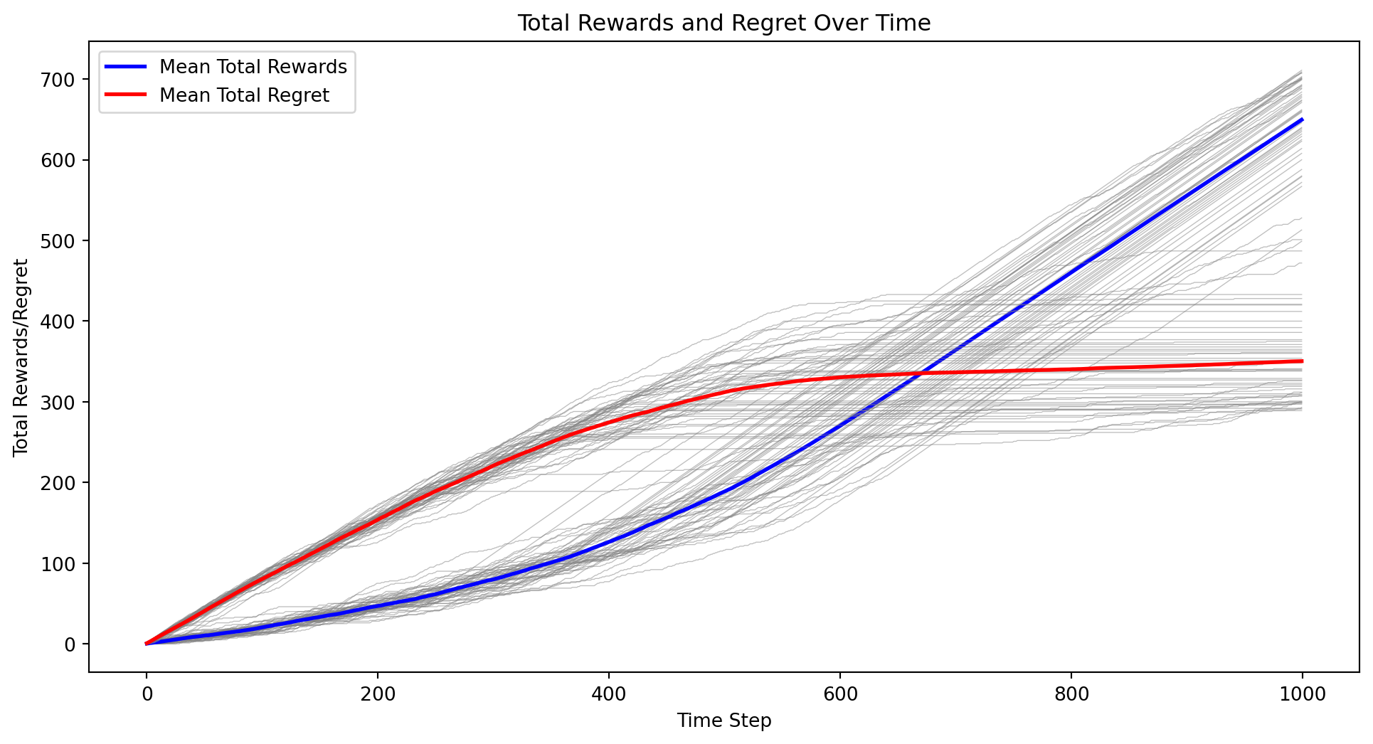
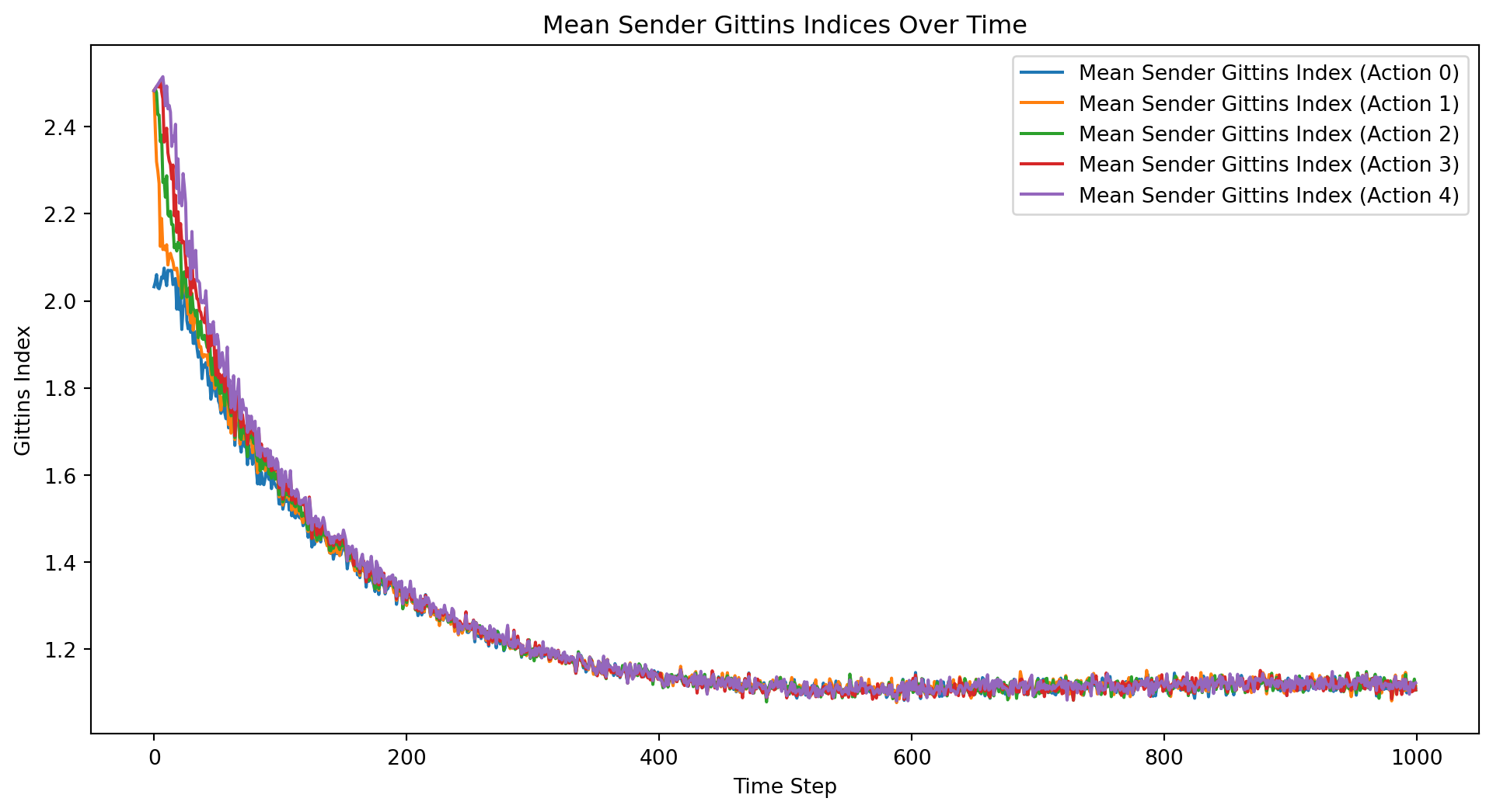
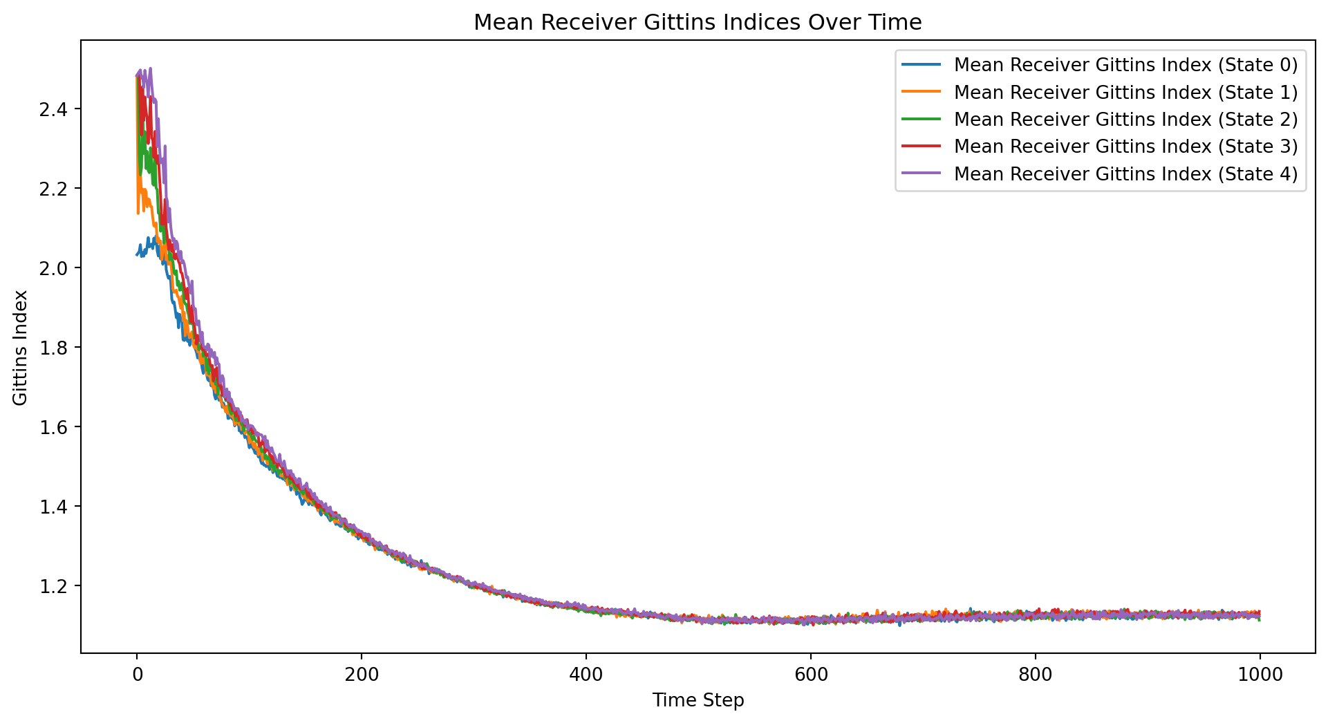
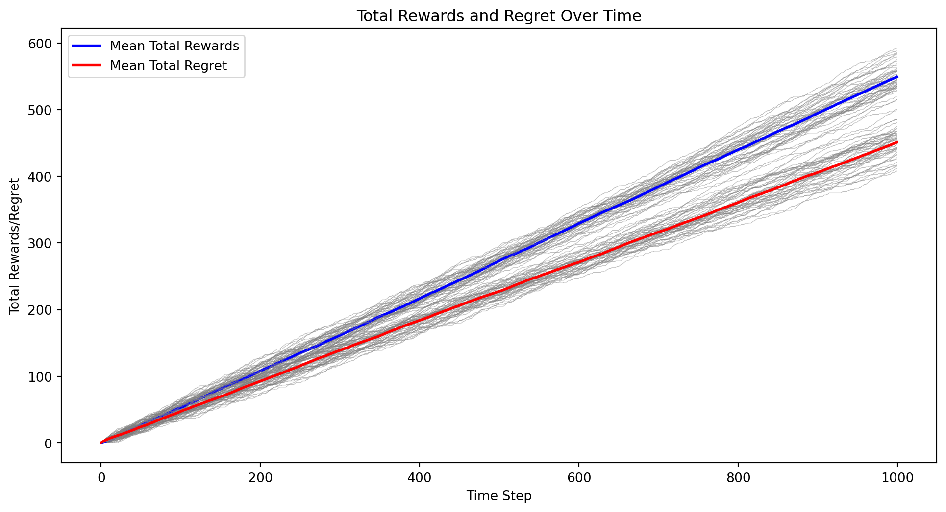
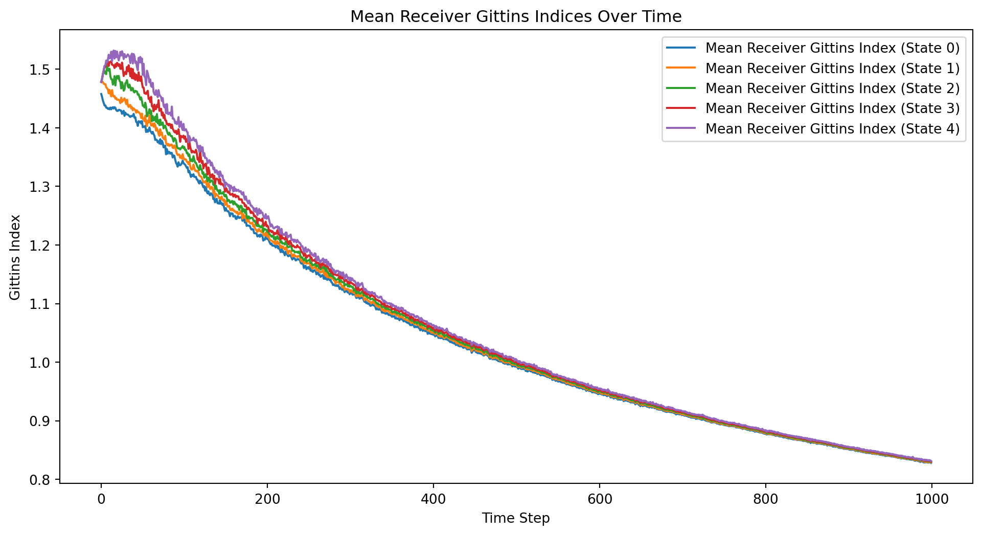
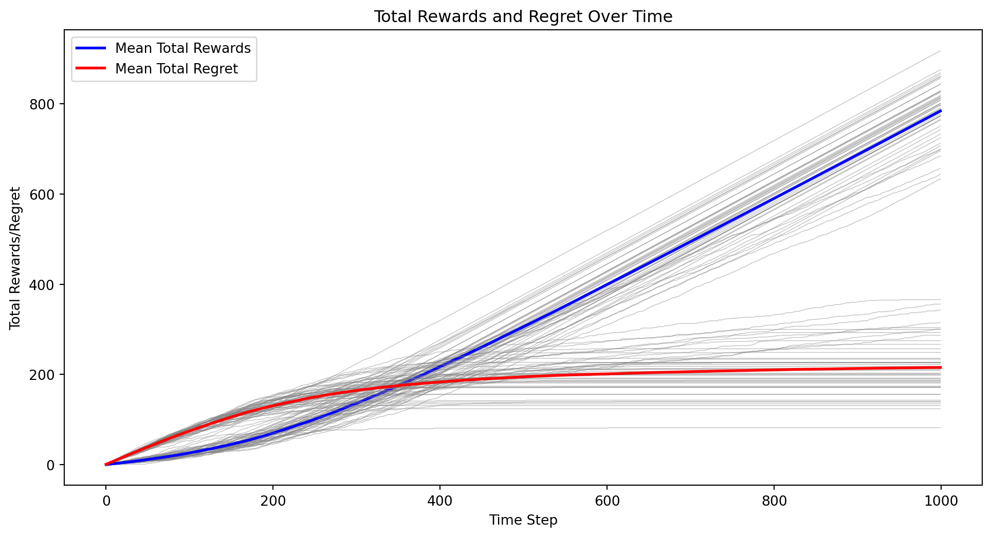
import numpy as np
import matplotlib.pyplot as plt

class BayesianContextualBandit:
    def __init__(self, n_states, n_actions):
        self.n_states = n_states
        self.n_actions = n_actions
        self.alpha = np.ones((n_states, n_actions))
        self.beta = np.ones((n_states, n_actions))

    def update(self, state, action, reward):
        if reward == 1:
            self.alpha[state, action] += 1
        else:
            self.beta[state, action] += 1

    def get_expected_reward(self, state, action):
        return self.alpha[state, action] / (self.alpha[state, action] + self.beta[state, action])

    def get_gittins_index(self, state, action):
        total_reward = self.alpha[state, action]
        total_count = self.alpha[state, action] + self.beta[state, action]
        return total_reward / total_count + np.sqrt(2 * np.log(np.sum(self.alpha + self.beta)) / total_count)

    def select_action(self, state):
        gittins_indices = [self.get_gittins_index(state, a) for a in range(self.n_actions)]
        return np.argmax(gittins_indices)

def sample_state(distribution, n_states):
    if distribution == "uniform":
        return np.random.randint(n_states)
    elif distribution == "normal":
        state = int(np.random.normal(loc=n_states/2, scale=n_states/6))
        return np.clip(state, 0, n_states - 1)
    else:
        raise ValueError("Unsupported distribution type")

def run_experiment(n_states, n_actions, n_iterations, state_distribution, k):
    all_rewards = np.zeros((k, n_iterations))
    all_regrets = np.zeros((k, n_iterations))
    all_sender_gittins_indices = np.zeros((k, n_actions, n_iterations))
    all_receiver_gittins_indices = np.zeros((k, n_states, n_iterations))
    
    for i in range(k):
        sender_bandit = BayesianContextualBandit(n_states, n_actions)
        receiver_bandit = BayesianContextualBandit(n_actions, n_states)
        
        total_reward = 0
        total_regret = 0
        
        for t in range(n_iterations):
            state = sample_state(state_distribution, n_states)
            sender_action = sender_bandit.select_action(state)
            receiver_action = receiver_bandit.select_action(sender_action)
            
            reward = 1 if receiver_action == state else 0
            total_reward += reward
            total_regret += 1 - reward
            
            all_rewards[i, t] = total_reward
            all_regrets[i, t] = total_regret
            
            sender_bandit.update(state, sender_action, reward)
            receiver_bandit.update(sender_action, receiver_action, reward)
            
            for action in range(n_actions):
                all_sender_gittins_indices[i, action, t] = sender_bandit.get_gittins_index(state, action)
            
            for s in range(n_states):
                all_receiver_gittins_indices[i, s, t] = receiver_bandit.get_gittins_index(sender_action, s)
    
    mean_rewards = np.mean(all_rewards, axis=0)
    mean_regrets = np.mean(all_regrets, axis=0)
    mean_sender_gittins_indices = np.mean(all_sender_gittins_indices, axis=0)
    mean_receiver_gittins_indices = np.mean(all_receiver_gittins_indices, axis=0)
    
    return all_rewards, all_regrets, mean_rewards, mean_regrets, mean_sender_gittins_indices, mean_receiver_gittins_indices

# Parameters
n_states = 5
n_actions = 5
n_iterations = 1000
state_distribution = "uniform"  # Change to "normal" for normal distribution
k = 50  # Number of experiment runs

# Run the experiment
all_rewards, all_regrets, mean_rewards, mean_regrets, mean_sender_gittins_indices, mean_receiver_gittins_indices = run_experiment(n_states, n_actions, n_iterations, state_distribution, k)

# Plot the mean total rewards and regrets over time along with individual curves
plt.figure(figsize=(12, 6))
for i in range(k):
    plt.plot(all_rewards[i], color='gray', alpha=0.5, linewidth=0.5)
plt.plot(mean_rewards, label='Mean Total Rewards', color='blue', linewidth=2)
for i in range(k):
    plt.plot(all_regrets[i], color='gray', alpha=0.5, linewidth=0.5)
plt.plot(mean_regrets, label='Mean Total Regret', color='red', linewidth=2)
plt.xlabel('Time Step')
plt.ylabel('Total Rewards/Regret')
plt.title('Total Rewards and Regret Over Time')
plt.legend()
plt.show()

# Plot the mean Gittins indices over time for the sender
plt.figure(figsize=(12, 6))
for action in range(n_actions):
    plt.plot(mean_sender_gittins_indices[action], label=f'Mean Sender Gittins Index (Action {action})')
plt.xlabel('Time Step')
plt.ylabel('Gittins Index')
plt.title('Mean Sender Gittins Indices Over Time')
plt.legend()
plt.show()

# Plot the mean Gittins indices over time for the receiver
plt.figure(figsize=(12, 6))
for state in range(n_states):
    plt.plot(mean_receiver_gittins_indices[state], label=f'Mean Receiver Gittins Index (State {state})')
plt.xlabel('Time Step')
plt.ylabel('Gittins Index')
plt.title('Mean Receiver Gittins Indices Over Time')
plt.legend()
plt.show()

Of course there is no reason to use independent probabilities for for learning.

The schemes described in the book condition state for the sender and on the signal for the receiver. I.E. a success for a signal/action pair implies:

a failure for the other state/signals options with the same states for the sender.
a failure for the other signal/action options with the same signal for the receiver.

In my algorithm I went further and added the logic that a success for a signals/action pair also implies:

a failure for the other state/signals options with the same signal but different states for the sender.
a failure for the other signal/action options with the same action but different signals for the receiver.

also implies that the signal wasn’t available for other states.

I’m not sure if there is a distribution that updates like that, though it isn’t that hard to implement either of the two schemes and they should work an extended beta distribution.

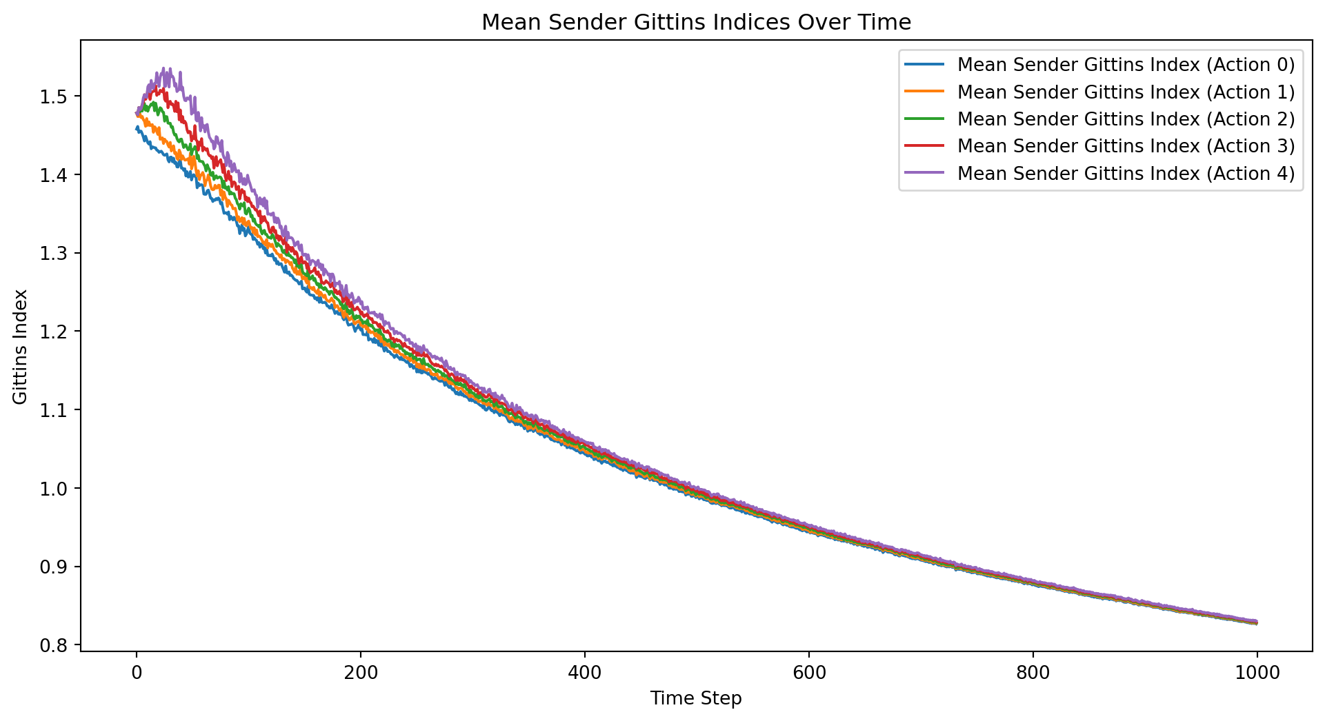
Derichlet-Multinomial variant

import numpy as np
import matplotlib.pyplot as plt

class BayesianContextualBandit:
    def __init__(self, n_states, n_actions):
        self.n_states = n_states
        self.n_actions = n_actions
        self.alpha = np.ones((n_states, n_actions))

    def update(self, state, action, reward):
        if reward == 1:
            self.alpha[state, action] += 1

    def get_expected_reward(self, state, action):
        alpha_sum = np.sum(self.alpha[state])
        return self.alpha[state, action] / alpha_sum

    def get_gittins_index(self, state, action):
        alpha_sum = np.sum(self.alpha[state])
        return self.alpha[state, action] / alpha_sum + np.sqrt(2 * np.log(alpha_sum) / (self.alpha[state, action] + 1))

    def select_action(self, state):
        gittins_indices = [self.get_gittins_index(state, a) for a in range(self.n_actions)]
        return np.argmax(gittins_indices)

def sample_state(distribution, n_states):
    if distribution == "uniform":
        return np.random.randint(n_states)
    elif distribution == "normal":
        state = int(np.random.normal(loc=n_states/2, scale=n_states/6))
        return np.clip(state, 0, n_states - 1)
    else:
        raise ValueError("Unsupported distribution type")

def run_experiment(n_states, n_actions, n_iterations, state_distribution, k):
    all_rewards = np.zeros((k, n_iterations))
    all_regrets = np.zeros((k, n_iterations))
    all_sender_gittins_indices = np.zeros((k, n_actions, n_iterations))
    all_receiver_gittins_indices = np.zeros((k, n_states, n_iterations))
    
    for i in range(k):
        sender_bandit = BayesianContextualBandit(n_states, n_actions)
        receiver_bandit = BayesianContextualBandit(n_actions, n_states)
        
        total_reward = 0
        total_regret = 0
        
        for t in range(n_iterations):
            state = sample_state(state_distribution, n_states)
            sender_action = sender_bandit.select_action(state)
            receiver_action = receiver_bandit.select_action(sender_action)
            
            reward = 1 if receiver_action == state else 0
            total_reward += reward
            total_regret += 1 - reward
            
            all_rewards[i, t] = total_reward
            all_regrets[i, t] = total_regret
            
            sender_bandit.update(state, sender_action, reward)
            receiver_bandit.update(sender_action, receiver_action, reward)
            
            for action in range(n_actions):
                all_sender_gittins_indices[i, action, t] = sender_bandit.get_gittins_index(state, action)
            
            for s in range(n_states):
                all_receiver_gittins_indices[i, s, t] = receiver_bandit.get_gittins_index(sender_action, s)
    
    mean_rewards = np.mean(all_rewards, axis=0)
    mean_regrets = np.mean(all_regrets, axis=0)
    mean_sender_gittins_indices = np.mean(all_sender_gittins_indices, axis=0)
    mean_receiver_gittins_indices = np.mean(all_receiver_gittins_indices, axis=0)
    
    return all_rewards, all_regrets, mean_rewards, mean_regrets, mean_sender_gittins_indices, mean_receiver_gittins_indices

# Parameters
n_states = 5
n_actions = 5
n_iterations = 1000
state_distribution = "uniform"  # Change to "normal" for normal distribution
k = 50  # Number of experiment runs

# Run the experiment
all_rewards, all_regrets, mean_rewards, mean_regrets, mean_sender_gittins_indices, mean_receiver_gittins_indices = run_experiment(n_states, n_actions, n_iterations, state_distribution, k)

# Plot the mean total rewards and regrets over time along with individual curves
plt.figure(figsize=(12, 6))
for i in range(k):
    plt.plot(all_rewards[i], color='gray', alpha=0.5, linewidth=0.5)
plt.plot(mean_rewards, label='Mean Total Rewards', color='blue', linewidth=2)
for i in range(k):
    plt.plot(all_regrets[i], color='gray', alpha=0.5, linewidth=0.5)
plt.plot(mean_regrets, label='Mean Total Regret', color='red', linewidth=2)
plt.xlabel('Time Step')
plt.ylabel('Total Rewards/Regret')
plt.title('Total Rewards and Regret Over Time')
plt.legend()
plt.show()

# Plot the mean Gittins indices over time for the sender
plt.figure(figsize=(12, 6))
for action in range(n_actions):
    plt.plot(mean_sender_gittins_indices[action], label=f'Mean Sender Gittins Index (Action {action})')
plt.xlabel('Time Step')
plt.ylabel('Gittins Index')
plt.title('Mean Sender Gittins Indices Over Time')
plt.legend()
plt.show()

# Plot the mean Gittins indices over time for the receiver
plt.figure(figsize=(12, 6))
for state in range(n_states):
    plt.plot(mean_receiver_gittins_indices[state], label=f'Mean Receiver Gittins Index (State {state})')
plt.xlabel('Time Step')
plt.ylabel('Gittins Index')
plt.title('Mean Receiver Gittins Indices Over Time')
plt.legend()
plt.show()

Thompson sampling

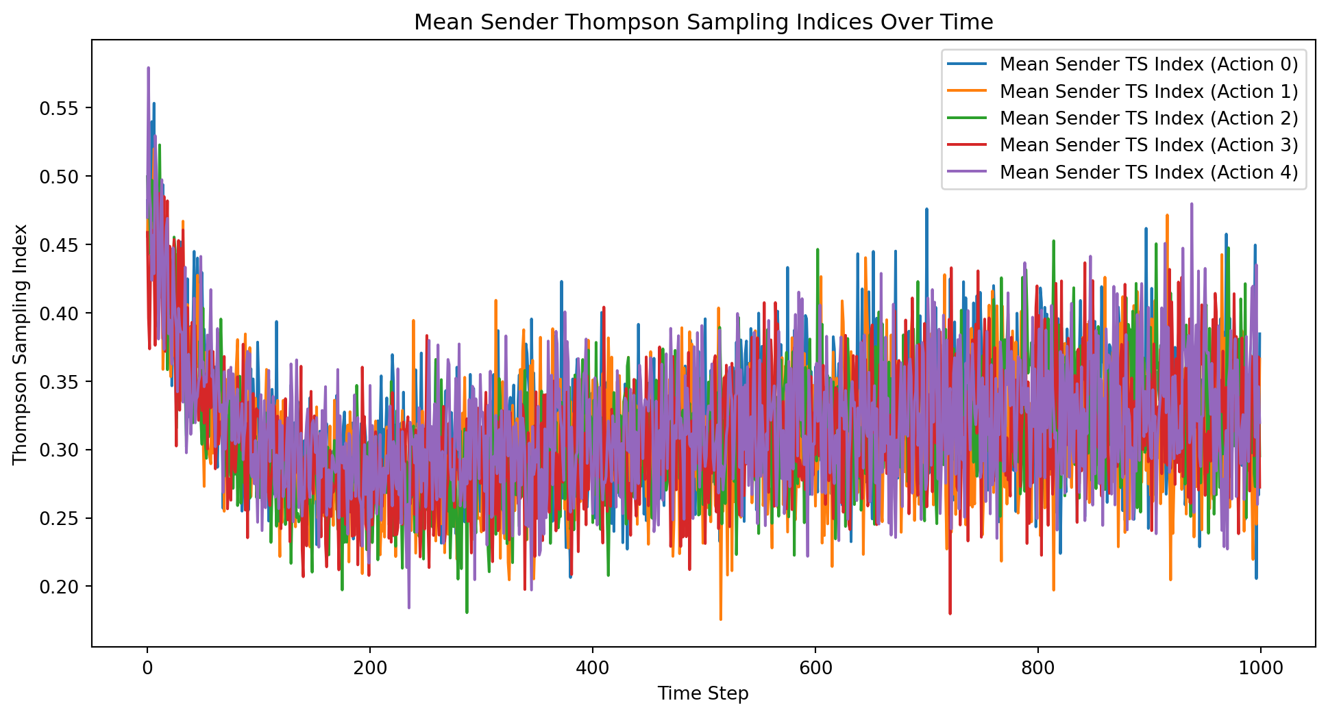
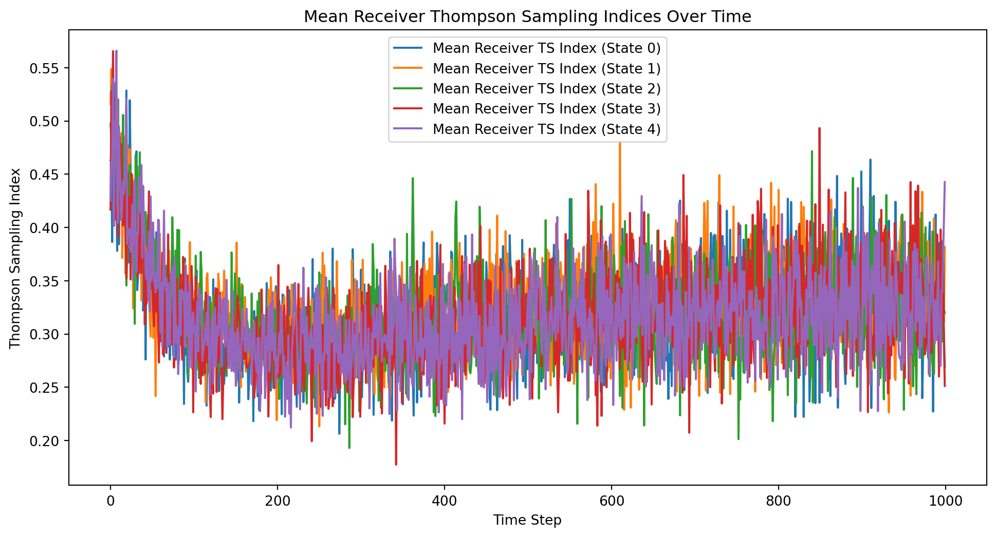
import numpy as np
import matplotlib.pyplot as plt

class ThompsonSamplingContextualBandit:
    def __init__(self, n_states, n_actions):
        self.n_states = n_states
        self.n_actions = n_actions
        self.alpha = np.ones((n_states, n_actions))
        self.beta = np.ones((n_states, n_actions))

    def update(self, state, action, reward):
        if reward == 1:
            self.alpha[state, action] += 1
        else:
            self.beta[state, action] += 1

    def select_action(self, state):
        samples = [np.random.beta(self.alpha[state, a], self.beta[state, a]) for a in range(self.n_actions)]
        return np.argmax(samples)

def sample_state(distribution, n_states):
    if distribution == "uniform":
        return np.random.randint(n_states)
    elif distribution == "normal":
        state = int(np.random.normal(loc=n_states/2, scale=n_states/6))
        return np.clip(state, 0, n_states - 1)
    else:
        raise ValueError("Unsupported distribution type")

def run_experiment(n_states, n_actions, n_iterations, state_distribution, k):
    all_rewards = np.zeros((k, n_iterations))
    all_regrets = np.zeros((k, n_iterations))
    all_sender_ts_indices = np.zeros((k, n_actions, n_iterations))
    all_receiver_ts_indices = np.zeros((k, n_states, n_iterations))
    
    for i in range(k):
        sender_bandit = ThompsonSamplingContextualBandit(n_states, n_actions)
        receiver_bandit = ThompsonSamplingContextualBandit(n_actions, n_states)
        
        total_reward = 0
        total_regret = 0
        
        for t in range(n_iterations):
            state = sample_state(state_distribution, n_states)
            sender_action = sender_bandit.select_action(state)
            receiver_action = receiver_bandit.select_action(sender_action)
            
            reward = 1 if receiver_action == state else 0
            total_reward += reward
            total_regret += 1 - reward
            
            all_rewards[i, t] = total_reward
            all_regrets[i, t] = total_regret
            
            sender_bandit.update(state, sender_action, reward)
            receiver_bandit.update(sender_action, receiver_action, reward)
            
            for action in range(n_actions):
                all_sender_ts_indices[i, action, t] = np.random.beta(sender_bandit.alpha[state, action], sender_bandit.beta[state, action])
            
            for s in range(n_states):
                all_receiver_ts_indices[i, s, t] = np.random.beta(receiver_bandit.alpha[sender_action, s], receiver_bandit.beta[sender_action, s])
    
    mean_rewards = np.mean(all_rewards, axis=0)
    mean_regrets = np.mean(all_regrets, axis=0)
    mean_sender_ts_indices = np.mean(all_sender_ts_indices, axis=0)
    mean_receiver_ts_indices = np.mean(all_receiver_ts_indices, axis=0)
    
    return all_rewards, all_regrets, mean_rewards, mean_regrets, mean_sender_ts_indices, mean_receiver_ts_indices

# Parameters
n_states = 5
n_actions = 5
n_iterations = 1000
state_distribution = "uniform"  # Change to "normal" for normal distribution
k = 50  # Number of experiment runs

# Run the experiment
all_rewards, all_regrets, mean_rewards, mean_regrets, mean_sender_ts_indices, mean_receiver_ts_indices = run_experiment(n_states, n_actions, n_iterations, state_distribution, k)

# Plot the mean total rewards and regrets over time along with individual curves
plt.figure(figsize=(12, 6))
for i in range(k):
    plt.plot(all_rewards[i], color='gray', alpha=0.5, linewidth=0.5)
plt.plot(mean_rewards, label='Mean Total Rewards', color='blue', linewidth=2)
for i in range(k):
    plt.plot(all_regrets[i], color='gray', alpha=0.5, linewidth=0.5)
plt.plot(mean_regrets, label='Mean Total Regret', color='red', linewidth=2)
plt.xlabel('Time Step')
plt.ylabel('Total Rewards/Regret')
plt.title('Total Rewards and Regret Over Time')
plt.legend()
plt.show()

# Plot the mean Thompson Sampling indices over time for the sender
plt.figure(figsize=(12, 6))
for action in range(n_actions):
    plt.plot(mean_sender_ts_indices[action], label=f'Mean Sender TS Index (Action {action})')
plt.xlabel('Time Step')
plt.ylabel('Thompson Sampling Index')
plt.title('Mean Sender Thompson Sampling Indices Over Time')
plt.legend()
plt.show()

# Plot the mean Thompson Sampling indices over time for the receiver
plt.figure(figsize=(12, 6))
for state in range(n_states):
    plt.plot(mean_receiver_ts_indices[state], label=f'Mean Receiver TS Index (State {state})')
plt.xlabel('Time Step')
plt.ylabel('Thompson Sampling Index')
plt.title('Mean Receiver Thompson Sampling Indices Over Time')
plt.legend()

plt.show()

Citation

BibTeX citation:

@online{bochman2024,
  author = {Bochman, Oren},
  title = {Roth {Erev} Learning in {Lewis} Signaling Games},
  date = {2024-09-17},
  url = {https://orenbochman.github.io/posts/2024/2024-05-09-RE-RL/re-rel.html},
  langid = {en}
}

For attribution, please cite this work as:

Bochman, Oren. 2024. “Roth Erev Learning in Lewis Signaling Games.” September 17, 2024. https://orenbochman.github.io/posts/2024/2024-05-09-RE-RL/re-rel.html.