Multilevel (hierarchical) modeling is a generalization of linear and generalized linear modeling in which regression coefficients are themselves given a model, whose parameters are also estimated from data. We illustrate the strengths and limitations of multilevel modeling through an example of the prediction of home radon levels in U.S. counties. The multilevel model is highly effective for predictions at both levels of the model, but could easily be misinterpreted for causal inference. Gelman, A. (2006).

Fundamental Concepts:

What is the difference between fixed effect, random effect and mixed effect models?

Under the Fixed Effect model we assume that the true effect size for all individuals is identical, and the only reason the effect size varies between studies is sampling error (error in estimating the effect size). Fixed effects are estimated using least squares (or, more generally, maximum likelihood)
Under the Random Effect or Population Average Effects* model we assume that the true effect size varies for each individuals and has a population statistic. random effects are estimated with shrinkage (“linear unbiased prediction” in the terminology of Robinson, 1991)
Multilevel (hierarchical) models get their name from their functional form which relates higher level features depend on the lower level ones.
Pooling
Shrinkage AKA Partial-Pooling county specific means are pulled toward the population mean. More generally shrinkage is predictions shifting towards the population average. See Shrinkage in Mixed Effects Models
Smoothing of uncertainty: Uncertainty about the county-specific means is lower (sometimes much lower) than if these parameters were estimated independently. (Better than the non-pooling model)
Proportional borrowing of information: Shrinkage and uncertainty reduction do not occur uniformly - information-poor counties must borrow a great deal of information from the other counties, while information-rich counties do not.
non-IID or Multicolinearity - Multilevel models can handle data at different levels that would be
Homoscedasticity of the data can be handled by the model (when gradients are allowed to vary).

The Data

This is based on the dataset from ‘Radon contamination’ (Gelman and Hill 2006). Radon is a radiactive gas that is a by product of radioactive decay of uranium within the soil. The EPA did a study of radon levels in 80,000 houses. The two important predictors are:

Measurement in the basement or the first floor (radon higher in basements)
County uranium level (positive correlation with radon levels).

The ‘natural’ hierarchy in the data is:

the state
county level,
house.

In these different models we are considering how to share information on within and between groups. This sharing of data is called pooling and is a type of learning mechanism. (It is the same pooling from game theory’s pooling equilibrium.)

One way to organize the different models is by increasing number of parameters.

Plate notation remainder:

Recall that plate notation is used in bayesian graphical model with repeating entities:

arrows indicate a dependency relation.
filled nodes are observed variables.
empty nodes are latent variables
small nodes are parameters
nodes in plates/boxes with index = N repeat N times.

Complete Pooling Model:

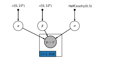
This is the simplest of all where one treat all counties the same, and estimate a single radon level.

The is a parametric model with 2 parameters, with alpha giving state wide radon level at the basements and \beta the adjustment for going up a floor (there are only two floor and beta is the gradient associated with drop of levels when going up a floor.)

y_i=\alpha + \beta x_i + \epsilon_i

where:

i is the house number (919)
x is the floor of the house
y log radon level
\alpha is the intercept parameter corresponding to a base radon level. In this model it’s a fixed effect across all counties.
\beta gradient parameter - corresponding to drop of radon level between floors. Again it’s a fixed effect across all counties.
\epsilon is an error term may represent measurement error, temporal within-house variation, or variation among houses.

the model model:

\alpha ~ N(0,10^5)
\beta ~ N(0,10^5)
\sigma ~ HalfCauchy(0,5)
y_i ~ $N(+ x_i,^2) $

The main issue with this model is that is ignores variation between counties. When we pool our data, we lose the information that different data points came from different counties. This means that each radon-level observation is sampled from the same probability distribution. Such a model fails to learn any variation in the sampling unit that is inherent within a group (e.g. a county). It only accounts for sampling variance.

Non-Pooling Model:

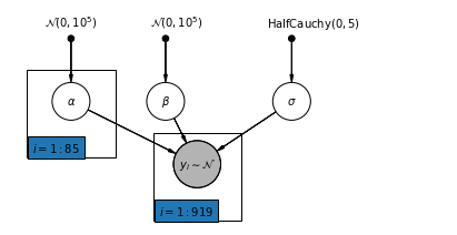
Model radon in each county independently.

y_i=\alpha_{j[i]} + \beta x_{j[i]} + \epsilon_i

where where:

j is the county number (1,…,85)
i is the house number (1,…,919) - though just the ones in the county
x is the floor of the house
y log radon measurement
\alpha intercept or bias parameter
\beta gradient parameter
\epsilon error term

we model:

[ \alpha_j ~ N(0,10^5) for j in counties]
[ y_i ~ $N $ for i in houses ] with parameters:
- \beta ~ N(0,10^5)
- \sigma ~ HalfCauchy(0,5)

providing us with a parametric model with 920 parameters.

Next one would use MCMC to learn which parameters minimize the total error.

The main issue with this model is that there are lots of parameters and in some counties very few point to estimate them. (for some just two). The unpolled estimates are difficult to trust.

When we analyze data unpooled, we imply that they are sampled independently from separate models. At the opposite extreme from the pooled case, this approach claims that differences between sampling units are too large to combine them:

Multilevel and Hierarchical models

Partial Pooling

In a hierarchical model, parameters are viewed as a sample from a population distribution of parameters considering them as neither entirely different or exactly the same. This is known as partial pooling.

recall: y_i=\alpha_{j[i]} + \beta x_{j[i]} + \epsilon_i

we now want to estimate an county level using a weighed average between the county level and the over all level average. \hat{\alpha}_j \approx \frac{(n_j/\sigma_y^2)\bar{y}_j + (1/\sigma_{\alpha}^2)\bar{y}}{(n_j/\sigma_y^2) + (1/\sigma_{\alpha}^2)}

where where:

j is the county number (1,…,85)
i is the house number (1,…,919) - though just the ones in the county
y log radon measurement
\alpha intercept or bias parameter
\beta gradient parameter
\epsilon error term

we model:

[ \alpha_j ~ N(\mu_a,\sigma_a) for j in counties] with parameters:
- \mu_a ~ N(0,10^5)]
- \sigma_a ~ HalfCauchy(0,5)
[ y_i ~ $N $ for i in houses ] with parameters:
- \mu_y ~ N(0,10^5)] (ignored)
- \sigma_y ~ HalfCauchy(0,5)

With partial pooling one expects:

Estimates for counties with smaller sample sizes will shrink towards the state-wide average.
Estimates for counties with larger sample sizes will be closer to the unpooled county estimates.

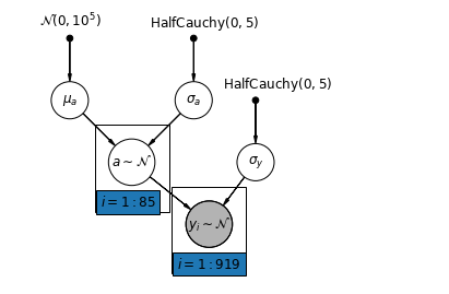
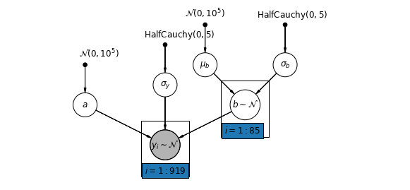
Varying Intercepts

We now a consider a more complex model that allows intercepts to vary across county, according to a random effect.

y_i = \alpha_{j[i]} + \beta x_{i} + \epsilon_i

where

\epsilon_i \sim N(0, \sigma_y^2)

and the intercept random effect:

\alpha_{j[i]} \sim N(\mu_{\alpha}, \sigma_{\alpha}^2)

The slope \beta, which lets the observation vary according to the location of measurement (basement or first floor), is still a fixed effect shared between different counties. As with the the unpooling model, we set a separate intercept for each county, but rather than fitting separate least squares regression models for each county, multilevel modeling shares strength among counties, allowing for more reasonable inference in counties with little data.

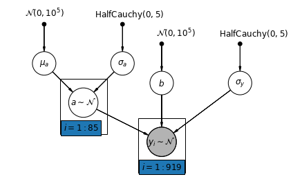
Varying Slopes

In this model, one posits that counties vary according to how the location of measurement (basement or first floor) influences the radon reading. In this case the intercept \alpha is shared between counties.

y_i = \alpha + \beta_{j[i]} x_{i} + \epsilon_i

j is the county number. (1,…,85)
i is the house number. (1,…,919) - though just the ones in the county
x (0 for basement 1 for 1st) floor of the house.
y log radon measurement
\alpha intercept parameter corresponding to a base radon level fixed across all counties.
\beta gradient parameter - corresponding to drop of radon level between floors
\epsilon_i error term considered at the house level.

Varying Intercepts and Slopes

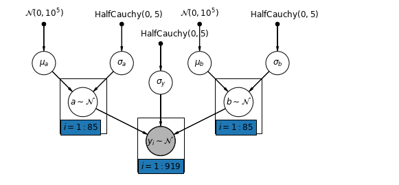
note: the plate model would be clearer if a and b were in the same plate making the level more explicit.

The most general model allows both the intercept and slope to vary by county:

y_i = \alpha_{j[i]} + \beta_{j[i]} x_{i} + \epsilon_i

where:

j is the county number. (1,…,85)
i is the house number. (1,…,919) - though just the ones in the county
x (0 for basement 1 for 1st) floor of the house.
y log radon measurement
\alpha_{ji} intercept parameter (corresponding to a base radon level) partially pooled across all counties.
\beta_{ji} gradient parameter (corresponding to drop of radon level between floors) partially pooled across all counties.
\epsilon_i error term considered at the house level.

Hierarchical Intercepts and Slopes

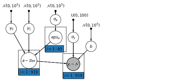
A primary strength of multilevel models is the ability to handle predictors on multiple levels simultaneously. If we consider the varying-intercepts model above:

y_i = \alpha_{j[i]} + \beta x_{i} + \epsilon_i

we may, instead of a simple random effect to describe variation in the expected radon value, specify another regression model with a county-level covariate. Here, we use the county uranium reading u_j, which is thought to be related to radon levels:

\alpha_j = \gamma_0 + \gamma_1 u_j + \zeta_j

\zeta_j \sim N(0,\sigma_{\alpha}^2)

Thus, we are now incorporating a house-level predictor (floor or basement) as well as a county-level predictor (uranium).

Note that the model has both indicator variables for each county, plus a county-level covariate.

In classical regression, this would result in collinearity. In a multilevel model, the partial pooling of the intercepts towards the expected value of the group-level linear model avoids this.

Group-level predictors also serve to reduce group-level variation \sigma_{\alpha}. An important implication of this is that the group-level estimate induces stronger pooling.

Correlation amongst levels

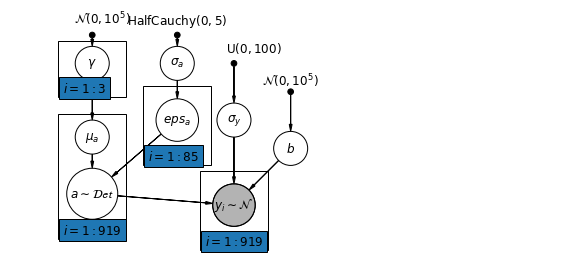
In some instances, having predictors at multiple levels can reveal correlation between individual-level variables and group residuals. We can account for this by including the average of the individual predictors as a covariate in the model for the group intercept.

\alpha_j = \gamma_0 + \gamma_1 u_j + \gamma_2 \bar{x} + \zeta_j

These are broadly referred to as contextual effects.

7 Conclusions

Benefits of Multilevel Models:

Accounting for natural hierarchical structure of observational data.
Estimation of coefficients for (under-represented) groups.
Incorporating individual- and group-level information when estimating group-level coefficients.
Allowing for variation among individual-level coefficients across groups.

References

Gelman, A., & Hill, J. (2006). Data Analysis Using Regression and Multilevel/Hierarchical Models (1st ed.). Cambridge University Press.
Gelman, A. (2006). Multilevel (Hierarchical) modeling: what it can and cannot do. Technometrics, 48(3), 432–435.

Citation

BibTeX citation:

@online{bochman2021,
  author = {Bochman, Oren},
  title = {Multilevel {Models}},
  date = {2021-05-16},
  url = {https://orenbochman.github.io/posts/2021/2021-05-16-mulitlevel-models/2021-05-16-mulitlevel-models.html},
  langid = {en}
}

For attribution, please cite this work as:

Bochman, Oren. 2021. “Multilevel Models.” May 16, 2021. https://orenbochman.github.io/posts/2021/2021-05-16-mulitlevel-models/2021-05-16-mulitlevel-models.html.