Evolutionary Games and Population Dynamics Summary

I’ve recently come across a book called “Evolutionary Games and Population Dynamics” by Josef Hofbauer and Karl Sigmund.

This book is a comprehensive introduction to the mathematical theory of evolutionary games and population dynamics.

The book covers a wide range of topics, including the basic concepts of game theory, the dynamics of evolutionary games, and the mathematical analysis of population dynamics.

The book also includes numerous examples and exercises to help readers understand the material.

Although the boook is primarily grounded in differential equations, my interest is to try and implement the models using agent-based modeling. This should have a two fold benefit:

1. learn how the differential equations are implemented in agent-based models
2. see and apply the techniques used in the book for analysis these dynamic systems ` - Lyapanov functions
   • stability analysis
   • bifurcation analysis
   • sensitivity to initial conditions
   • identifying phase Boundries
   • etc.
3. create more realistic model with heterogeneous agents with spatial dynamics using ABM like Mesa and study them with the above tools
4. create interactive visualizations of phase space to help understand the dynamics of these systems
5. study parameter space to map out the different regions of the phase space.

I will be summarizing the key concepts from the book in this document.

Dynamical Systems and Lotka-Volterra Equations

Logistic Growth

Density Dependence

• competition
• mutualism
• host-parasite realtionshuip

Exponetial Growth

\dot x = Rx

Logistic Growth

\dot x = r x (1-\frac{x}{K})

x(t) = \frac{K}{1+(\frac{K}{x_0}-1)e^{-rt}}

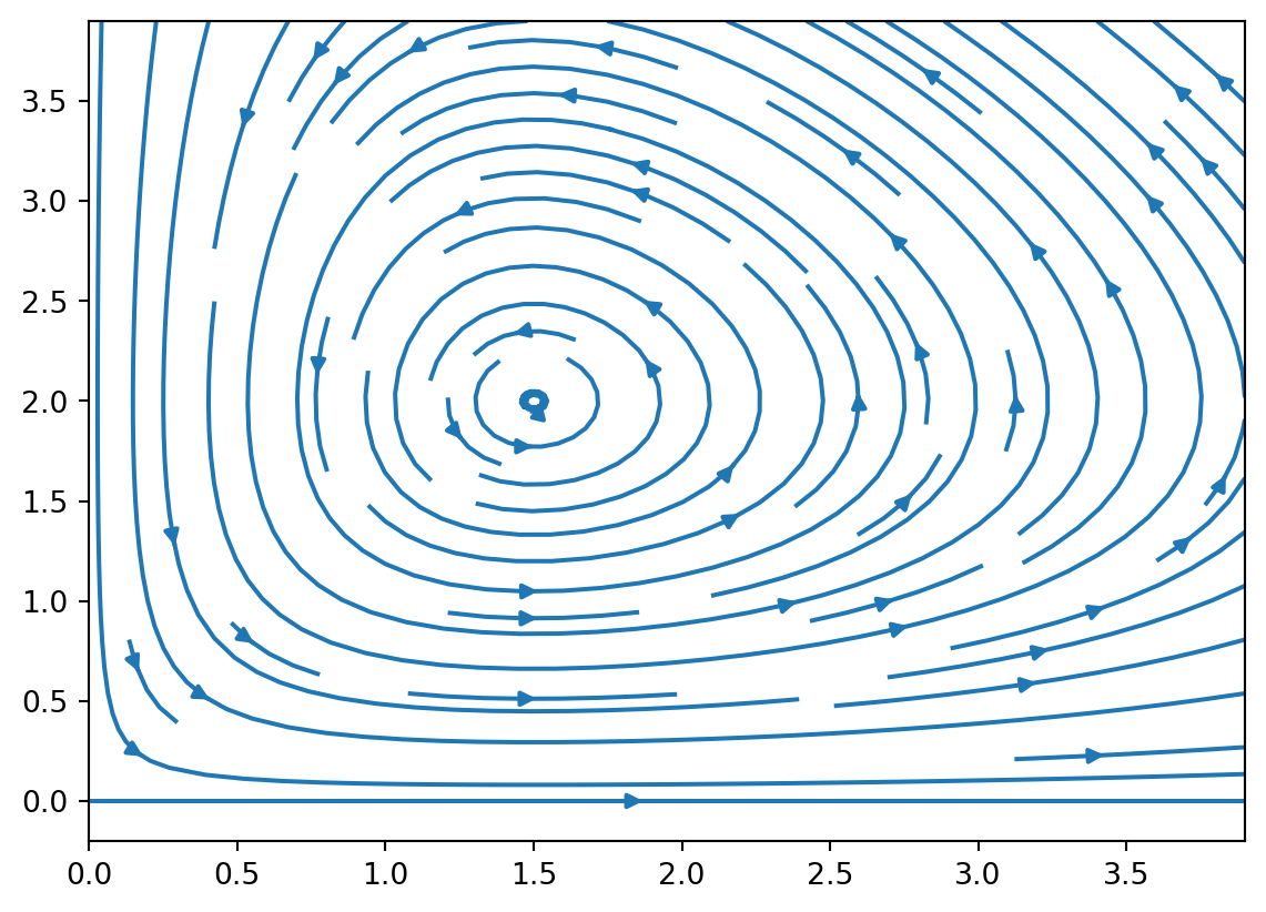
Lotka-Volterra equations for predator-prey systems

In the years after the First World War, the amouiif of predatory fish in the Adriatic was found to be considerably higher than in the years before.

Predator-Prey Model

Volterra assumed that the rate of growth of the prey population, in the absence of predators, is given by some constant a, but decreases linearly as a function of the density у of predators. This leads to x/x = a — by (with a,b> 0). In the absence of prey, the predatory fish would have to die, which means a negative rate of growth; but this rate picks up with the density χ of prey fish, hence y/y = — c + dx (with c,d > 0). Together, this yields

\begin{align*} \dot x &= x(\alpha - \beta y) \\ \dot y &= y(\delta x - \gamma )\\ \text{where} & \quad \alpha, \beta, \gamma, \delta > 0 \end{align*} \qquad here, x is the prey population (rabbits) and y is the predator population (fox).

phase space diagram

from pylab import *

alpha, beta, gamma, delta = 2, 1, 1.5, 1
xvalues, yvalues = meshgrid(arange(0, 4, 0.1), arange(0, 4, 0.1))
xdot = xvalues*(alpha - beta * yvalues)
ydot = yvalues *( delta * xvalues - gamma)
streamplot(xvalues, yvalues, xdot, ydot)
show()