Markov Chain models
Markov models consist of entities that can be in a set of states and there are transition probabilities between those states. e.g., there is a set of students. Those students could be in either one of two states, alert or bored. There is some probability P that they move from alert to bored and some probability Q that they move from bored to alert. Over time these students are moving back and forth from the alert state to the bored state. The Markov process gives us a framework to understand how those dynamics take place.
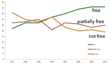
This can also be applied to countries being free, being partially free or not free. Historically there are different trends. The free states seem to be increasing. The not-free tend to be decreasing. The Markov process can be used to figure out where this is going to end up.
The Markov convergence theorem state that, as long as a couple of assumptions hold, namely that there is a finite number of states, and the transition probabilities stay fixed, and you can get from any state to any other state, then the system goes to equilibrium. This is a really powerful finding that has all sorts of implications.
To understand Markov processes, matrices can be used. Matrices are grids of numbers. Those numbers will be the transition probabilities. Multiplication by matrices is used to understand Markov processes and the Markov convergence theorem. These matrices can be used to explain why these systems go to equilibria.
Markov processes are interesting for two reasons. First, Markov processes are a useful way to think about how the world works and this gives powerful results The Markov convergence theorem says that these systems are going to equilibria. Second, is the idea of exaptation. That the Markov model is incredibly fertile and can be applied in a whole range of different settings. Transition probabilities and matrices can also be used in a lot of settings as well.
A simple Markov model
Let’s use the simple example of alert and bored students. Some percentage of the students are alert and some percentage of the students are bored. An alert student can switch and become bored and a bored student can switch and become alert. We need to assume something about the transition probabilities. Assume that in any given period, 20% of the alert students become bored, but 25% of the bored students become alert. Here the matrices will be useful.
We can calculate this by hand. Assume we start with 100 alert and 0 bored, so (A,B)->(100,0). After one period, you have 80 alert and 20 bored, so (A,B) -> (100-20+0=80, 0-0+20=20). If you go on then (A,B) -> (80-16+5=69, 20+16-5=31). This is rather complicated so there must be a better way to keep track of this.
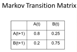
The Markov transition matrix gives the probabilities of moving from state to state. The columns tell what is true at time t and the rows tells what is true at time t+1. So if you’re alert at time t, there’s an 80% chance you stay alert, and a 20% chance you become bored. If you’re bored at time t, there’s a 25% chance you become alert and a 75% chance that you stay bored.
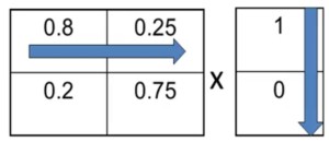
The calculation process works as follows. For each row you multiply the elements with the value at t to get the value at t+1. So A(t+1) = 0.8A(t) + 0.25B(t) and B(t+1) = 0.2A(t) + 0.75B(t). It is possible to repeat these steps. The result after six periods is that only 58% of the students are alert.
Where does this process stop? It is possible to do the same calculation starting with all students being bored. After 6 turns 53% is alert and 47% is bored. It looks like there is an equilibrium.
So how do we calculate the equilibrium? The equilibrium would mean that at t+1 the same percentage of people is alert as at t. So 0.8p + 0.25(1-p) = p => p/5 = (1-p)/4 => (4/5)p = 1 - p => (9/5)p = 1 => p = 5/9. So in equilibrium 5/9 will be alert and 4/9 will be bored. In that case 20% of the alert will get bored, which is 1/9, and 25% of the bored will become alert, which is also 1/9.
This is a stochastic equilibrium. The thing that doesn’t change is the probability. The population is still moving from alert to bored and from bored to alert.
Markov model of democratisation
A slightly more complicated model involves countries that can either be free, partly free or not free at all. This can be used to learn how Markov processes work, how they can be extended to more dimensions. Let’s start simply with just a two-state model with democracies and dictatorships. Assume that 5% of democracies become dictatorships every decade, and that 20% of dictatorships become democracies.
Let’s start off by assuming 30% are democracies and 70% are dictatorships. After a decade, (0.95 * 0.3 + 0.2 * 0.7) * 100% = 42.5% are going to be democracies while 57.5% will be dictatorships. One decade later, 52% will be democracies and 48% will be dictatorships. The equilibrium can also be calculated. 0.95p + 0.2(1-p) = p => 1/5 - p/5 = p/20 => p/4 = 1/5 => p = 4/5. The surprising finding is that we only end up with 80% democracies even though 95% of democracies stay democracies and 20% of dictatorships become democracies in each decade.
A sophisticated model is having three categories, free, partly free, and not free. This data comes from Freedom House and shows an increase in free countries and a decrease in not free countries, and a slight decrease in partly free countries. What is likely to happen?
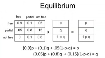
You can use five year increments, use transition probabilities, and do some crude estimates. This results in the following. Each decade, 5% of free, and 15% of not free become partly free. And 5% of not free and 10% of partly free become free. And 10% of partly free become not free.
This is a three by three matrix. With computers it is possible to make a huge matrices and solve them for equilibrium. So what does that equilibrium look like? All we do is take each one of these rows, and multiply by the columns. The algebra results in 62.5% of countries being free, 25% being partly free, and 12.5% being not free, presuming that the transition probabilities stay fixed.
The model shows some general trends. The graph generated from the model doesn’t look exactly the same as the real picture, but it doesn’t look bad either. The model comes up at the end of the 40 year period with values that are close to those in the real world but that is because the estimated transition probabilities were based on the actual data. What’s more interesting is that the patterns look fairly similar as well.
Markov convergence theorem
The Markov convergence theorem tells that, provided a few fairly mild assumptions are met, Markov processes converge to a stochastic equilibrium. There are movements, but the probability of being in each state stays fixed. The conditions that must hold for that to be true are the following:
- a finite number of states
- fixed transition probabilities
- eventually you can get from any state to any other state
- not a simple cycle
If these conditions hold then a Markov process converges to an equilibrium distribution that is unique, which means that there is only one equilibrium distribution that is independent of the initial state. It is determined entirely by the transition probabilities. In Markov processes, the initial state, history, and interventions to change the state have no effect on the long run on the system.
Interventions can have effect. First, it could take a long time before the system is back to equilibrium so that an intervention may have a significant benefit. Second, some of the conditions of the theorem may not hold in the real world, most notably the fixed transition probabilities. The transition probabilities may change over time as the function of the state of the system. Changing the state has a temporary effect, but changing the transition probabilities has permanent consequences. Useful interventions change the transition probabilities. This may happen to tipping points.
Expectation of the Markov model
The Markov model can be used in contexts and problems we never would have thought of. The first way is taking the entire process and modelling to other things. The second way is using a part of the Markov model, the transition probability matrix, to understand some things that are surprising and interesting. A Markov process is. Fixed set of states with fixed transition probabilities between those states. If it is possible to get from any state to any other through a sequence of transitions, then the Markov convergence theorem states that the process is going to a unique equilibrium.
This can be applied to voter turnout. Assume that there is a set of voters at time t, and there is a set a of non-voters at time t. We can make a transition matrix of that to find out how many are going to vote at time t+1, and how many are not going to vote at time t+1. If the transition probabilities stay fixed then there is a unique equilibrium that tells the number of people that is expected to vote in any election. This can also be applied to school attendance as each day there are children that go to school and children that don’t go to school. These two applications are very standard.
It is also possible to use only a part of the Markov model, the Markov transition matrix, to identify writers. The transition matrix can be used to figure out who wrote a book. So suppose some anonymous person wrote a book and you are trying to figure out whether Bob or Elisa wrote it.
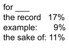
You can figure out transition probabilities by taking some key words, and then create transition matrices. e.g., you can calculate at what percentage of the time does “the record”, “example” or “the sake of” of follow the word “for”. You can compare this with books Bob and Elisa wrote with the use of computers.
This can be applied to medical diagnosis and treatment. Typically, there’s a sequence of reactions to that treatment. You can write down transition probabilities that can be multi-stage. e.g., if the treatment is going to be successful, the patient goes through the following transitions: first pain, then feeling slightly depressed, then some more pain, but then the patient gets better. Alternatively, if the treatment is not successful, it could be that, initially the patient is depressed, then there is mild pain, then there’s no pain, and then the treatment fails. This can be used to figure out early on whether or not a treatment will be successful.
Another example is the road to war. Suppose there are two countries and there is some tension. The political process goes through the following transitions. First there are some political statements on each side, then that leads to trade embargoes, followed by military buildup. Based on this sequence of three events, you estimate the likelihood of war based on historical data of previous times when those three transitions happened.
In these cases we are not using the full power of the Markov model and we do not assume that the transition probabilities necessarily stay fixed. We are not interested in solving for the equilibrium. All we’re trying to do is just use this probability matrix to organize the data in such a way that we can think more clearly about what’s likely to happen.
References
Note: this page is based on the following source:
- (Page 2014) MOOC, Course material & Transcripts.
- TA Notes by (Fisher 2014).
- Student notes by in (Klein Ikink 2016) and (Groh 2017).
Reuse
Citation
@online{bochman2023,
  author = {Bochman, Oren},
  title = {Lesson 10 - {Markov} {Processes}},
  date = {2023-08-10},
  url = {https://orenbochman.github.io/notes/model_thinking/w10.html},
  langid = {en}
}
