Reading: Adaptive Mixtures of Local Experts
TLDR
Serial ensambles like bagging operate using a cooperative loss function for the ensemble. Parallel ensembles should use a competitive loss function for the ensamle. Neural networks are slow to train and are best combined in parallel. The paper considers the type of losses function that promotes.
Over Views
- In (Nowlan and Hinton 1990), the authors offer a fascinating insights into the mechanics of ensembling, which is the approach of aggregating several lower capacity models into a single high capacity model.
- The ensembling is a form of the divide and conquer heuristic.
- Bagging uses a parallel approach where we average the outcomes. By Fisher’s fundamental theorem of natural selection the more diverse the models in an ensemble the faster it will the ensemble will learn.
- Boosting uses a sequential approach - each subsequent model works on the residual of the previous
- In the course, Hinton make the case that when ensembling neural networks one should use competition, rather than the cooperative approach that is the basis of bagging and boosting submodels.
- The big idea here is to get the sub model to specialize thus getting the ML system to converge faster.
- Converging faster means shorter training time or
- Getting the same results on a smaller dataset — and not having enough data is a common problem.
- Mixture of experts involves lots of overhead and so it is an approach we see less often. It is a way of squeezing more accuracy out of an ML model and so it tends to re-surface when a problem has matured and people are looking for small gains from better ML ops.
Abstract
“We present a new supervised learning procedure for systems composed of many separate networks, each of which learns to handle a subset of the complete set of training cases. The new procedure can be viewed either as a modular version of a multilayer supervised network, or as an associative version of competitive learning. It therefore provides a new link between these two apparently different approaches. We demonstrate that the learning procedure divides up a vowel discrimination task into appropriate subtasks, each of which can be solved by a very simple expert network.”
My Notes:
This paper is the first time I read about ensembles - and was an introduction. I would later read much more in Intorduction to statistical learning using R1. As time goes by ensembles keep getting more of my attention. We put them to work in setting that provides higher capacity models for small data setting. Also, the gating network is like a meta model which may be adapted to quantify uncertainty for each expert at the training case level.
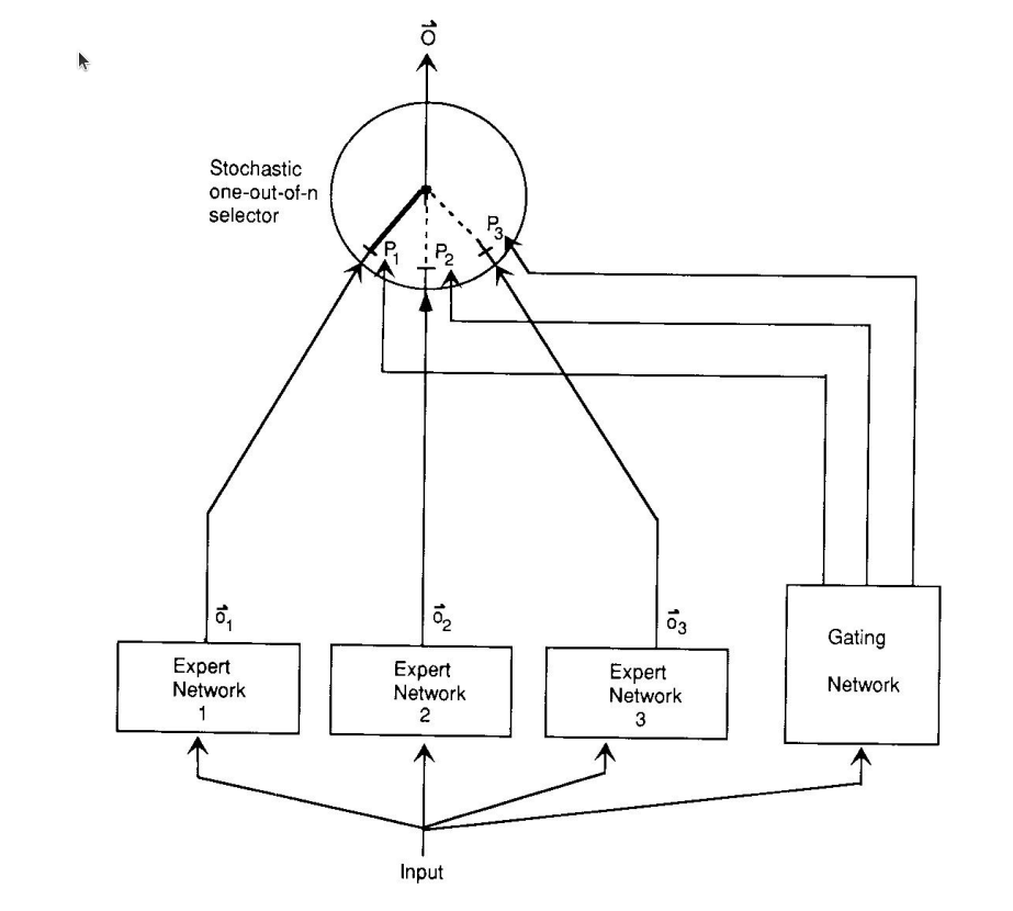
The architecture shown bellow uses expert networks trained on a vowel discrimination (classification) task alongside a gating network whose responsibility is to pick the best classifier for the input.
I had been familiar with the idea that the gating network is responsible to convert the output of the experts to the actual experts. It turns out that the gating network also needs to learn which expert is better on a given type of input, and that it also controls the data expert get. This allocation can be hard (each training case goes to one expert) or soft (several experts are allocated). I also noted that some of the prior work was authored by Bastro, the leading authority on Reinforcement Learning. In prior work the gating network the learn to allocate training cases to one or a few expert - which allows them specialize (the weights are decoupled) also learns to The earlier idea is to utilize or learn to partition the training data so that one can train specialized models that are local experts on the problem space and then use some linear combination of the expert’s predictions to make predictions. But using such a linear combination requires that the expert cancel each other’s output.
A cooperative loss function
E^c= ||\vec{d^c} -\sum_i p_i^c \vec o_i^c||^2 \tag{1}
where :
- \vec o_i^c is the output vector of expert i on case c.
- \vec d_c is the desired output for case c.
The authors say that the cooperative loss function in (1) foster an unwanted coupling between the experts, in the sense that a change in one expert’s weights will create a residual loss seen by the other experts in (1). This leads to cooperation but each expert has learn to neutralize the residual it sees from the others experts. So in both cases all models contribute to the inference, instead of just one or a few, which is counter to the idea of being an expert on a subset of the data.
The first competitive loss function
In (Jacobs et al. 1991) the authors used a hard selection mechanism by modifying the objective function to encourage competition and foster greater specialization by using only activate one expert at a time. This paper suggest that it is enough to modify the loss so that the experts compete. The idea being that “the selector acts as a multiple input, single output stochastic switch; the probability that the switch will select the output from expert j is p_j governed by:
E^c = <||\vec d^c - \vec o^c ||> =\sum_i\ p_i^c||\vec d^c- \vec o_i||^2 \tag{2}
where :
p_j = \frac{e^{x_j}}{\sum_i e^x_i}
soon we are shown a much better loss function:
The second competitive loss function
does not encourage cooperation rather than specialization, which required using many experts in each prediction. Later work added penalty terms in the objective function to gate a single active exert in the prediction. Jacobs, Jordan, and Barton, 1990. The paper offers an alternative error function that encourages specialization.
The difference difference between the error functions.
The second competitive error function
E^c= -log\sum_i\ p_i^c e^{\frac{1}{2}||d^c- \vec o_i||^2} \tag{3}
Why the second loss is more competitive?
The error defined in Equation 2 is simply the negative log probability of generating the desired output vector under the mixture of Gaussian’s model described at the end of the next section.
To see why this error function works better, it is helpful to compare the derivatives of the two error functions with respect to the output of an expert. From from Equation 2 we get:
\frac {\partial E^c}{\partial \vec o_i^c} = -2p_i^c(\vec d^c-\vec o_c^c) \tag{4}
while the derivative from Equation 3 gives us:
\frac {\partial E^c}{\partial \vec o_i^c} = -\bigg[\frac{p_i^c e^{\frac{1}{2}||d^c- \vec o_i||^2}}{\sum_j p_j^c e^{\frac{1}{2}||d^c- \vec o_j||^2}}\bigg](\vec d^c-\vec o_c^c) \tag{5}
In Equation 4 the term \vec p^c_i is used to weigh the derivative for expert i, while in equation 5 the weighting term takes into account how well expert i does relative to other experts, which is a more useful measure of the relevance of expert i to training case c, especially early in the training. Suppose, that the gating network initially gives equal weights to all experts and ||d^c-\vec o_j||>1 for all the experts. Equation 4 will adapt the best-fitting expert the slowest, whereas Equation 5 will adapt it the fastest.
Making the learning associative
If two loss function are not enough, the authors now suggest a third loss function. This loss looks at the distance from the average vector. logP^c= -log\sum_i\ p_i^c K e^{-\frac{1}{2}||\vec\mu_i- \vec o^c||^2} \tag{6}
My wrap up 🎬
I may not fully grasped all the ideas behind this loss and it requires reading additional papers as it was not covered in the lectures. The results parts compares number of epochs needed for different models ensembles and neural networks to reach some level of accuracy on the validation set. The application is also rather complex, but the vowel clustering task itself seems rather simple.
I was glad I went over this aper as the notions of faster training, competitive loss, associative learning seem to resurface in rather varied contexts2 and knowing this results and paper is a decent starting point in the area.
References
Footnotes
Reuse
Citation
@online{bochman2017,
  author = {Bochman, Oren},
  title = {Deep {Neural} {Networks} -\/-\/- {Readings} {I} for {Lesson}
    10},
  date = {2017-10-02},
  url = {https://orenbochman.github.io/notes/dnn/dnn-10/r1.html},
  langid = {en}
}