Lecture 7a: Modeling sequences: A brief overview
This video talks about some advanced material that will make a lot more sense after you complete the course: it introduces some generative models for unsupervised learning (see video 1e), namely Linear Dynamical Systems and Hidden Markov Models. These are neural networks, but they’ve very different in nature from the deterministic feed forward networks that we’ve been studying so far. For now, don’t worry if those two models feel rather mysterious.
However, Recurrent Neural Networks are the next topic of the course, so make sure that you understand them.
Getting targets when modeling sequences
- When applying machine learning to sequences, we often want to turn an input sequence into an output sequence that lives in a different domain.
- E. g. turn a sequence of sound pressures into a sequence of word identities.
- When there is no separate target sequence, we can get a teaching signal by trying to predict the next term in the input sequence.
- The target output sequence is the input sequence with an advance of 1 step.
- This seems much more natural than trying to predict one pixel in an image from the other pixels, or one patch of an image from the rest of the image.
- For temporal sequences there is a natural order for the predictions.
- Predicting the next term in a sequence blurs the distinction between supervised and unsupervised learning.
- It uses methods designed for supervised learning, but it doesn’t require a separate teaching signal.
Memoryless models for sequences
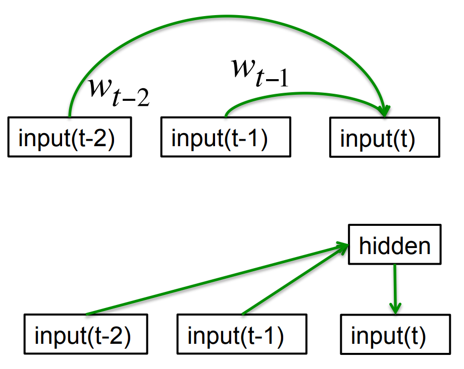
- Autoregressive models Predict the next term in a sequence from a fixed number of previous terms using “delay taps”.
- Feed-forward neural nets These generalize autoregressive models by using one or more layers of non-linear hidden units. e.g. Bengio’s first language model.
Beyond memoryless models
- If we give our generative model some hidden state, and if we give this hidden state its own internal dynamics, we get a much more interesting kind of model.
- It can store information in its hidden state for a long time.
- If the dynamics is noisy and the way it generates outputs from its hidden state is noisy, we can never know its exact hidden state.
- The best we can do is to infer a probability distribution over the space of hidden state vectors.
- This inference is only tractable for two types of hidden state model.
- The next three slides are mainly intended for people who already know about these two types of hidden state model. They show how RNNs differ.
- Do not worry if you cannot follow the details.
Linear Dynamical Systems (engineers love them!)
- These are generative models. They have a realvalued hidden state that cannot be observed directly.
- The hidden state has linear dynamics with Gaussian noise and produces the observations using a linear model with Gaussian noise.
- There may also be driving inputs.
- To predict the next output (so that we can shoot down the missile) we need to infer the hidden state.
- A linearly transformed Gaussian is a Gaussian. So the distribution over the hidden.
A fundamental limitation of HMMs
- Consider what happens when a hidden Markov model generates data.
- At each time step it must select one of its hidden states. So with N hidden states it can only remember log(N) bits about what it generated so far.
- Consider the information that the first half of an utterance contains about the second half:
- The syntax needs to fit (e.g. number and tense agreement).
- The semantics needs to fit. The intonation needs to fit.
- The accent, rate, volume, and vocal tract characteristics must all fit.
- All these aspects combined could be 100 bits of information that the first half of an utterance needs to convey to the second half. 2^100
Recurrent neural networks
- RNNs are very powerful, because they combine two properties:
- Distributed hidden state that allows them to store a lot of information about the past efficiently.
- Non-linear dynamics that allows them to update their hidden state in complicated ways.
- With enough neurons and time, RNNs can compute anything that can be computed by your computer.
Do generative models need to be stochastic?
- Linear dynamical systems and hidden Markov models are stochastic models.
- But the posterior probability distribution over their hidden states given the observed data so far is a deterministic function of the data.
- Recurrent neural networks are deterministic.
- So think of the hidden state of an RNN as the equivalent of the deterministic probability distribution over hidden states in a linear dynamical system or hidden Markov model. ## Recurrent neural networks
- What kinds of behaviour can RNNs exhibit?
- They can oscillate. Good for motor control?
- They can settle to point attractors. Good for retrieving memories?
- They can behave chaotically. Bad for information processing?
- RNNs could potentially learn to implement lots of small programs that each capture a nugget of knowledge and run in parallel, interacting to produce very complicated effects.
- But the computational power of RNNs makes them very hard to train.
- For many years we could not exploit the computational power of RNNs despite some heroic efforts (e.g. Tony Robinson’s speech recognizer).
Lecture 7b: Training RNNs with back propagation
Most important prerequisites to perhaps review: videos 3d and 5c (about backprop with weight sharing).
After watching the video, think about how such a system can be used to implement the brain of a robot as it’s producing a sentence of text, one letter at a time.
What would be input; what would be output; what would be the training signal; which units at which time slices would represent the input & output?
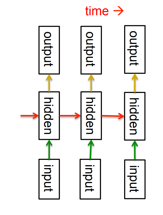
The equivalence between feedforward nets and recurrent nets
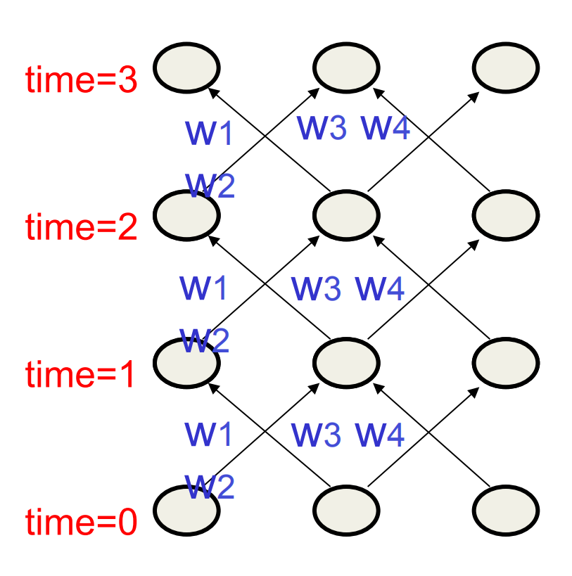
Assume that there is a time delay of 1 in using each connection.
The recurrent net is just a layered net that keeps reusing the same weights.
Reminder: Backpropagation with weight constraints
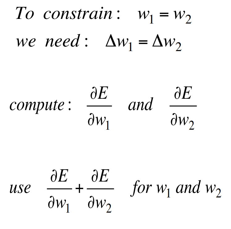
- It is easy to modify the backprop algorithm to incorporate linear constraints between the weights.
- We compute the gradients as usual, and then modify the gradients so that they satisfy the constraints.
- So if the weights started off satisfying the constraints, they will continue to satisfy them.
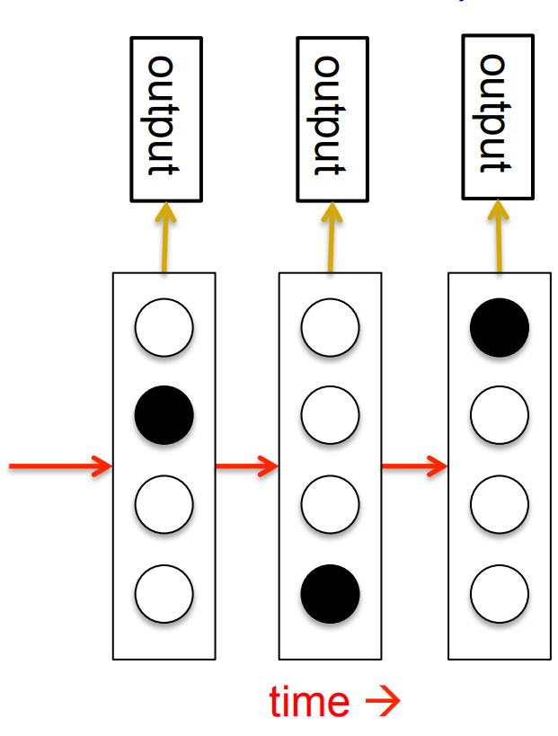
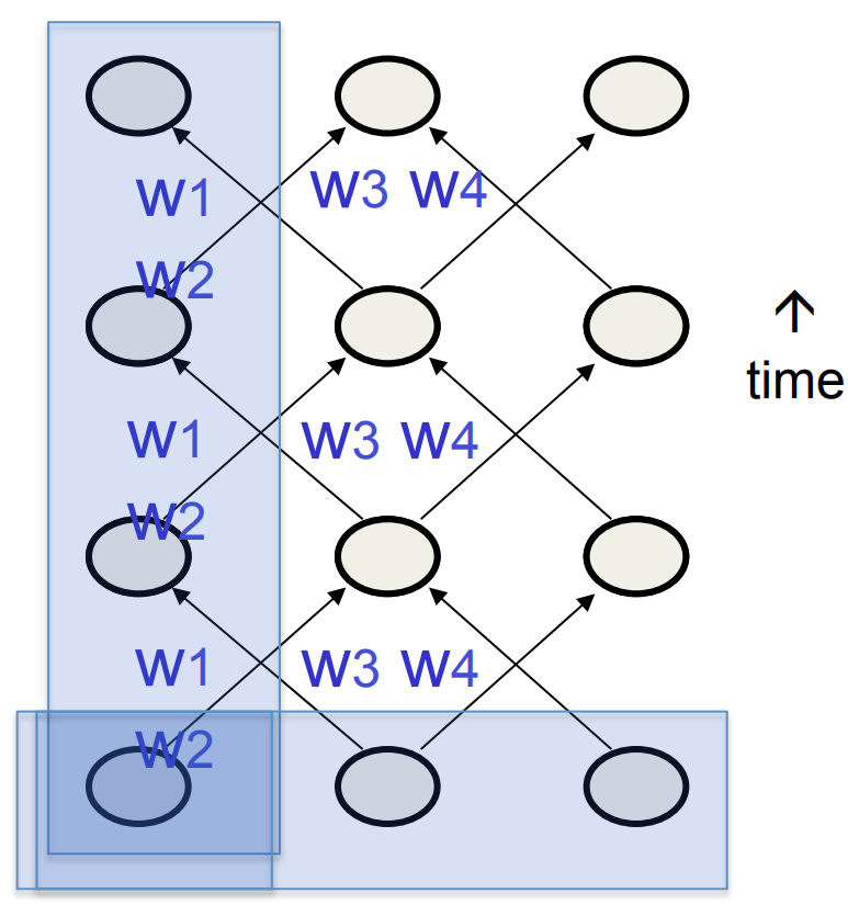
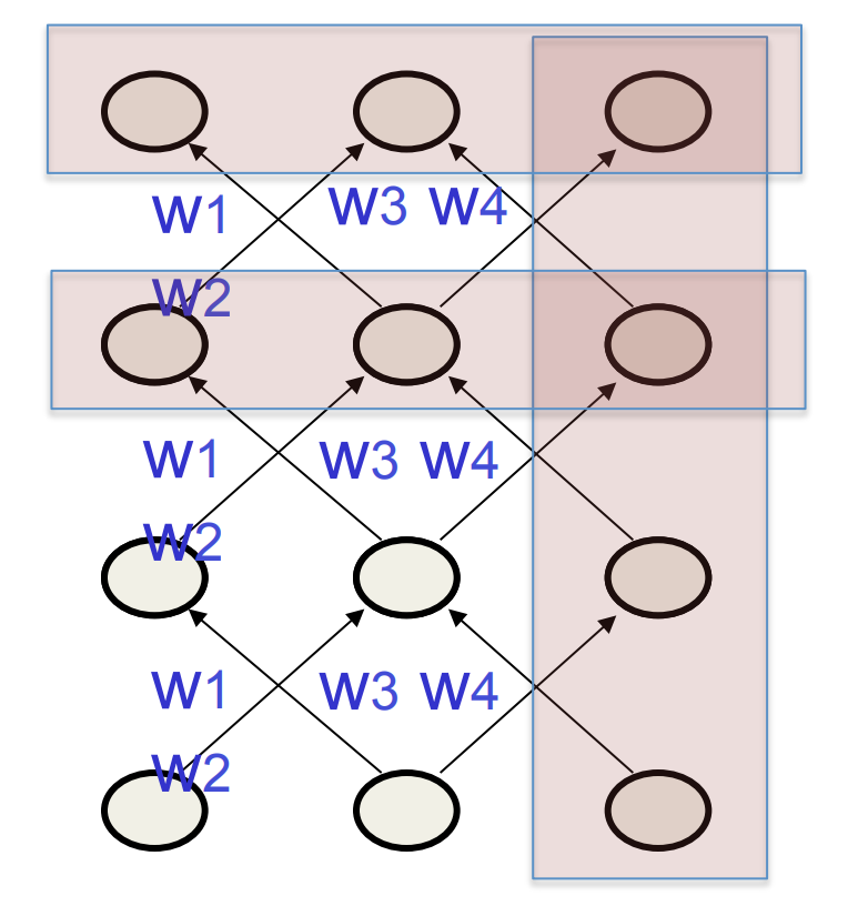
Backpropagation through time
- We can think of the recurrent net as a layered, feed-forward net with shared weights and then train the feed-forward net with weight constraints.
- We can also think of this training algorithm in the time domain:
- The forward pass builds up a stack of the activities of all the units at each time step.
- The backward pass peels activities off the stack to compute the error derivatives at each time step.
- After the backward pass we add together the derivatives at all the different times for each weight.
An irritating extra issue
- We need to specify the initial activity state of all the hidden and output units.
- We could just fix these initial states to have some default value like 0.5.
- But it is better to treat the initial states as learned parameters.
- We learn them in the same way as we learn the weights.
- Start off with an initial random guess for the initial states.
- At the end of each training sequence, backpropagate through time all the way to the initial states to get the gradient of the error function with respect to each initial state.
- Adjust the initial states by following the negative gradient.
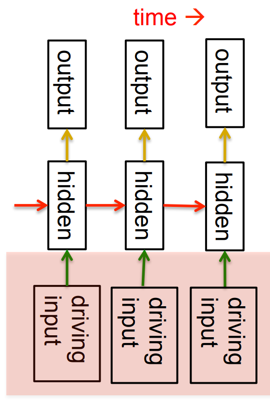
Providing input to recurrent networks
- We can specify inputs in several ways:
- Specify the initial states of all the units.
- Specify the initial states of a subset of the units.
- Specify the states of the same subset of the units at every time step.
- This is the natural way to model most sequential data.
Teaching signals for recurrent networks
- We can specify targets in several ways:
- Specify desired final activities of all the units
- Specify desired activities of all units for the last few steps
- Good for learning attractors
- It is easy to add in extra error derivatives as we backpropagate.
- Specify the desired activity of a subset of the units.
- The other units are input or hidden units.
Lecture 7c: A toy example of training an RNN
Clarification at 3:33: there are two input units. Do you understand what each of those two is used for?
The hidden units, in this example, as in most neural networks, are logistic. That’s why it’s somewhat reasonable to talk about binary states: those are the extreme states.
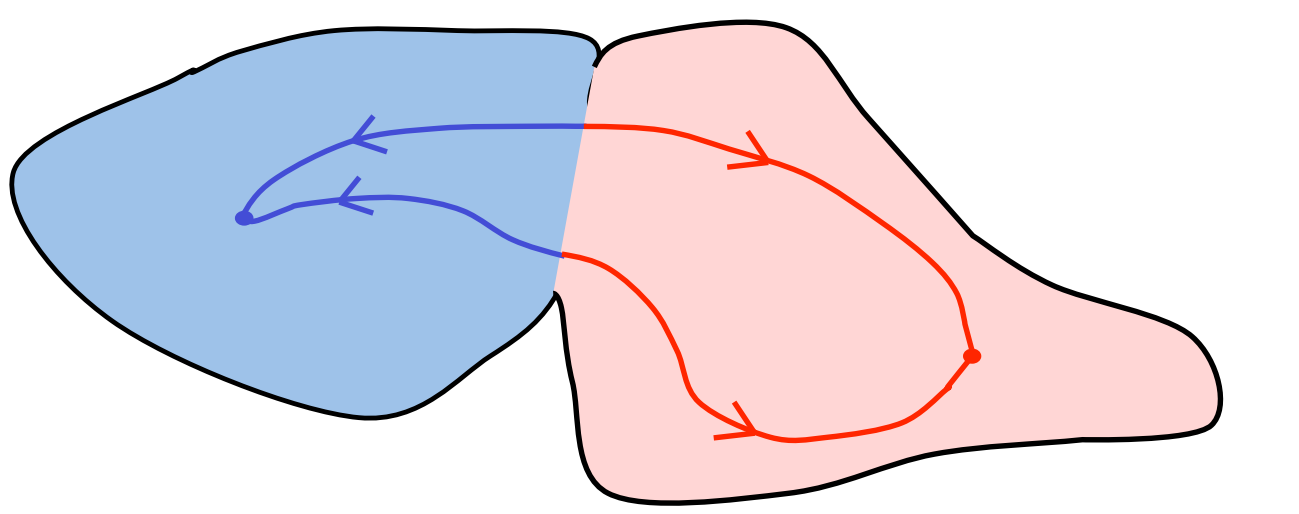
A good toy problem for a recurrent network
:::  :::
:::
- We can train a feedforward net to do binary addition, but there are obvious regularities that it cannot capture efficiently.
- We must decide in advance the maximum number of digits in each number.
- The processing applied to the beginning of a long number does not generalize to the end of the long number because it uses different weights.
- As a result, feedforward nets do not generalize well on the binary addition task.
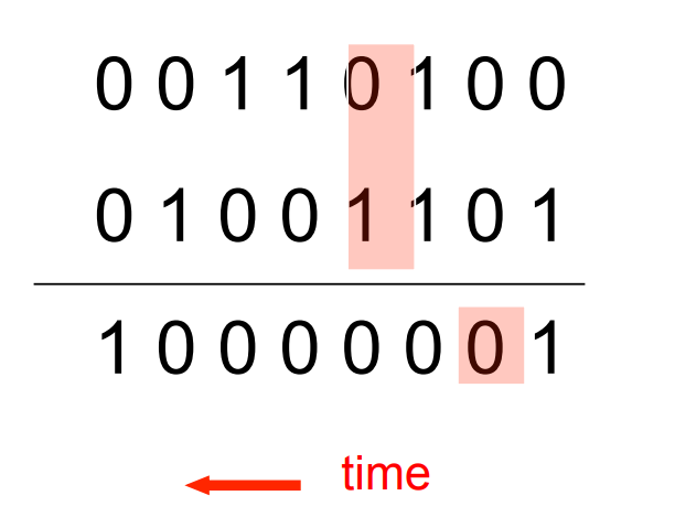
The algorithm for binary addition

This is a finite state automaton. It decides what transition to make by looking at the next column. It prints after making the transition. It moves from right to left over the two input numbers.
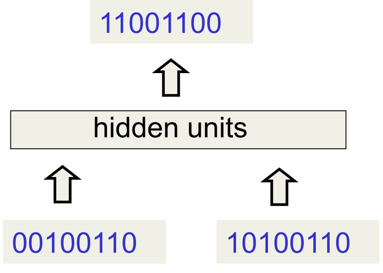
A recurrent net for binary addition
- The network has two input units and one output unit.
- It is given two input digits at each time step.
- The desired output at each time step is the output for the column that was provided as input two time steps ago.
- It takes one time step to update the hidden units based on the two input digits.
- It takes another time step for the hidden units to cause the output
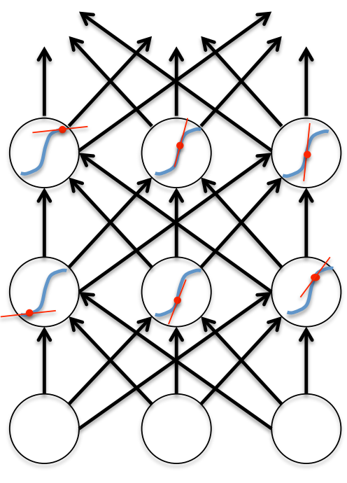
The connectivity of the network
The 3 hidden units are fully interconnected in both directions. - This allows a hidden activity pattern at one time step to vote for the hidden activity pattern at the next time step. - The input units have feedforward connections that allow then to vote for the next hidden activity pattern.
What the network learns
- It learns four distinct patterns of activity for the 3 hidden units. These patterns correspond to the nodes in the finite state automaton.
- Do not confuse units in a neural network with nodes in a finite state automaton. Nodes are like activity vectors.
- The automaton is restricted to be in exactly one state at each time. The hidden units are restricted to have exactly one vector of activity at each time.
- A recurrent network can emulate a finite state automaton, but it is exponentially more powerful. With N hidden neurons it has 2^N possible binary activity vectors (but only N^2 weights)
- This is important when the input stream has two separate things going on at once.
- A finite state automaton needs to square its number of states.
- An RNN needs to double its number of units.
Lecture 7d: Why it is difficult to train an RNN
This is all about backpropagation with logistic hidden units. If necessary, review video 3d and the example that we studied in class.
Remember that Geoffrey explained in class how the backward pass is like an extra long linear network? That’s the first slide of this video.
Echo State Networks: At 6:36, “oscillator” describes the behavior of a hidden unit (i.e. the activity of the hidden unit oscillates), just like we often use the word “feature” to functionally describe a hidden unit.
Echo State Networks: like when we were studying perceptrons, the crucial question here is what’s learned and what’s not learned. ESNs are like perceptrons with randomly created inputs.
At 7:42: the idea is good initialization with subsequent learning (using backprop’s gradients and stochastic gradient descent with momentum as the optimizer).
The backward pass is linear
 - There is a big difference between the forward and backward passes. - In the forward pass we use squashing functions (like the logistic) to prevent the activity vectors from exploding. - The backward pass, is completely linear. If you double the error derivatives at the final layer, all the error derivatives will double. - The forward pass determines the slope of the linear function used for backpropagating through each neuron.
The problem of exploding or vanishing gradients
- What happens to the magnitude of the gradients as we backpropagate through many layers?
- If the weights are small, the gradients shrink exponentially.
- If the weights are big the gradients grow exponentially.
- Typical feed-forward neural nets can cope with these exponential effects because they only have a few hidden layers.
- In an RNN trained on long sequences (e.g. 100 time steps) the gradients can easily explode or vanish.
- We can avoid this by initializing the weights very carefully.
- Even with good initial weights, its very hard to detect that the current target output depends on an input from many time-steps ago.
- So RNNs have difficulty dealing with long-range dependencies.
Why the back-propagated gradient blows up
- If we start a trajectory within an attractor, small changes in where we start make no difference to where we end up.
- But if we start almost exactly on the boundary, tiny changes can make a huge difference.
Four effective ways to learn an RNN
- Long Short Term Memory Make the RNN out of little modules that are designed to remember values for a long time.
- Hessian Free Optimization: Deal with the vanishing gradients problem by using a fancy optimizer that can detect directions with a tiny gradient but even smaller curvature.
- The HF optimizer ( Martens & Sutskever, 2011) is good at this.
- Echo State Networks: Initialize the inputàhidden and hiddenàhidden and outputàhidden connections very carefully so that the hidden state has a huge reservoir of weakly coupled oscillators which can be selectively driven by the input.
- ESNs only need to learn the hiddenàoutput connections.
- Good initialization with momentum Initialize like in Echo State Networks, but then learn all of the connections using momentum.
Lecture 7e: Long-term Short-term-memory
This video is about a solution to the vanishing or exploding gradient problem. Make sure that you understand that problem first, because otherwise this video won’t make much sense.
The material in this video is quite advanced.
In the diagram of the memory cell, there’s a somewhat new type of connection: a multiplicative connection. It’s shown as a triangle.
It can be thought of as a connection of which the strength is not a learned parameter, but is instead determined by the rest of the neural network, and is therefore probably different for different training cases.
This is the interpretation that Mr Hinton uses when he explains backpropagation through time through such a memory cell.
That triangle can, alternatively, be thought of as a multiplicative unit: it receives input from two different places, it multiplies those two numbers, and it sends the product somewhere else as its output.
Which two of the three lines indicate input and which one indicates output is not shown in the diagram, but is explained.
In Geoffrey’s explanation of row 4 of the video, “the most active character” means the character that the net, at this time, consider most likely to be the next character in the character string, based on what the pen is doing.
Long Short Term Memory (LSTM)
- Hochreiter & Schmidhuber (1997) solved the problem of getting an RNN to remember things for a long time (like hundreds of time steps).
- They designed a memory cell using logistic and linear units with multiplicative interactions.
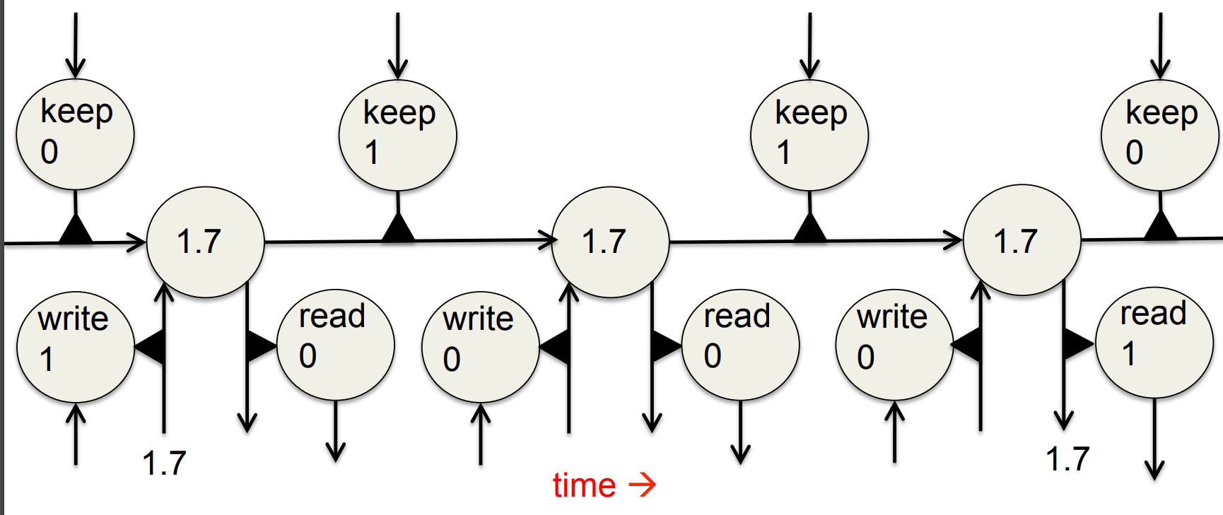
- Information gets into the cell whenever its “write” gate is on.
- The information stays in the cell so long as its “keep” gate is on.
- Information can be read from the cell by turning on its “read” gate.
Implementing a memory cell in a neural network
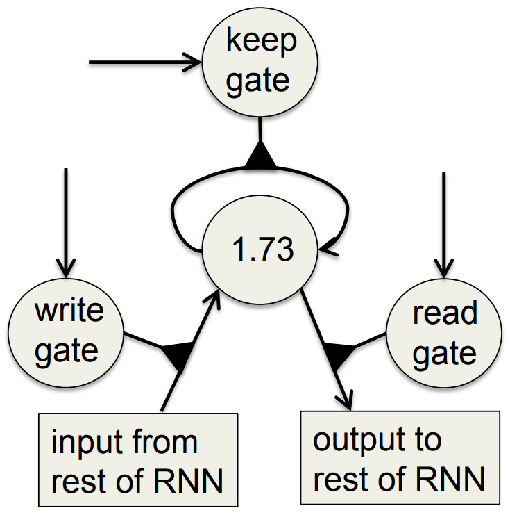
To preserve information for a long time in the activities of an RNN, we use a circuit that implements an analog memory cell. - A linear unit that has a self-link with a weight of 1 will maintain its state.
- Information is stored in the cell by activating its write gate. - Information is retrieved by activating the read gate. - We can backpropagate through this circuit because logistics are have nice derivatives.
Backpropagation through a memory cell
Reading cursive handwriting
- This is a natural task for an RNN.
- The input is a sequence of (x,y,p) coordinates of the tip of the pen, where p indicates whether the pen is up or down.
- The output is a sequence of characters.
- Graves & Schmidhuber (2009) showed that RNNs with LSTM are currently the best systems for reading cursive writing.
- They used a sequence of small images as input rather than pen coordinates. A demonstration of online handwriting recognition by an RNN with Long Short Term Memory (from Alex Graves)
- The movie that follows shows several different things:
- Row 1: This shows when the characters are recognized.
- It never revises its output so difficult decisions are more delayed.
- Row 2: This shows the states of a subset of the memory cells.
- Notice how they get reset when it recognizes a character.
- Row 3: This shows the writing. The net sees the x and y coordinates.
- Optical input actually works a bit better than pen coordinates.
- Row 4: This shows the gradient backpropagated all the way to the x and y inputs from the currently most active character.
- This lets you see which bits of the data are influencing the decision.
Reuse
Citation
@online{bochman2017,
  author = {Bochman, Oren},
  title = {Deep {Neural} {Networks} - {Notes} for {Lesson} 7},
  date = {2017-09-01},
  url = {https://orenbochman.github.io/notes/dnn/dnn-07/l_07.html},
  langid = {en}
}