Deep Neural Networks - Notes for Lesson 7d

Lecture 7d: Why it is difficult to train an RNN

This is all about backpropagation with logistic hidden units. If necessary, review video 3d and the example that we studied in class.

Remember that Geoffrey explained in class how the backward pass is like an extra long linear network? That’s the first slide of this video.

Echo State Networks: At 6:36, “oscillator” describes the behavior of a hidden unit (i.e. the activity of the hidden unit oscillates), just like we often use the word “feature” to functionally describe a hidden unit.

Echo State Networks: like when we were studying perceptrons, the crucial question here is what’s learned and what’s not learned. ESNs are like perceptrons with randomly created inputs.

At 7:42: the idea is good initialization with subsequent learning (using backprop’s gradients and stochastic gradient descent with momentum as the optimizer).

The backward pass is linear

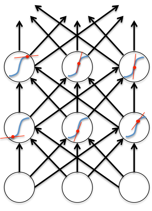- There is a big difference between the forward and backward passes. - In the forward pass we use squashing functions (like the logistic) to prevent the activity vectors from exploding. - The backward pass, is completely linear. If you double the error derivatives at the final layer, all the error derivatives will double. - The forward pass determines the slope of the linear function used for backpropagating through each neuron.

The problem of exploding or vanishing gradients

• What happens to the magnitude of the gradients as we backpropagate through many layers?
  • If the weights are small, the gradients shrink exponentially.
  • If the weights are big the gradients grow exponentially.
• Typical feed-forward neural nets can cope with these exponential effects because they only have a few hidden layers.
• In an RNN trained on long sequences (e.g. 100 time steps) the gradients can easily explode or vanish.
  • We can avoid this by initializing the weights very carefully.
• Even with good initial weights, its very hard to detect that the current target output depends on an input from many time-steps ago.
  • So RNNs have difficulty dealing with long-range dependencies.

Why the back-propagated gradient blows up

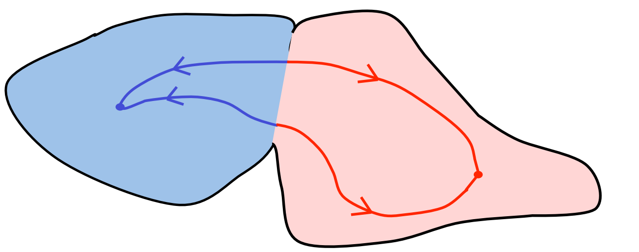
• If we start a trajectory within an attractor, small changes in where we start make no difference to where we end up.
• But if we start almost exactly on the boundary, tiny changes can make a huge difference.

Four effective ways to learn an RNN

• Long Short Term Memory Make the RNN out of little modules that are designed to remember values for a long time.
• Hessian Free Optimization: Deal with the vanishing gradients problem by using a fancy optimizer that can detect directions with a tiny gradient but even smaller curvature.
  • The HF optimizer ( Martens & Sutskever, 2011) is good at this.
• Echo State Networks: Initialize the inputàhidden and hiddenàhidden and outputàhidden connections very carefully so that the hidden state has a huge reservoir of weakly coupled oscillators which can be selectively driven by the input.
  • ESNs only need to learn the hiddenàoutput connections.
• Good initialization with momentum Initialize like in Echo State Networks, but then learn all of the connections using momentum.