Deep Neural Networks - Notes for Lesson 7b

Lecture 7b: Training RNNs with back propagation

Most important prerequisites to perhaps review: videos 3d and 5c (about backprop with weight sharing).

After watching the video, think about how such a system can be used to implement the brain of a robot as it’s producing a sentence of text, one letter at a time.

What would be input; what would be output; what would be the training signal; which units at which time slices would represent the input & output?

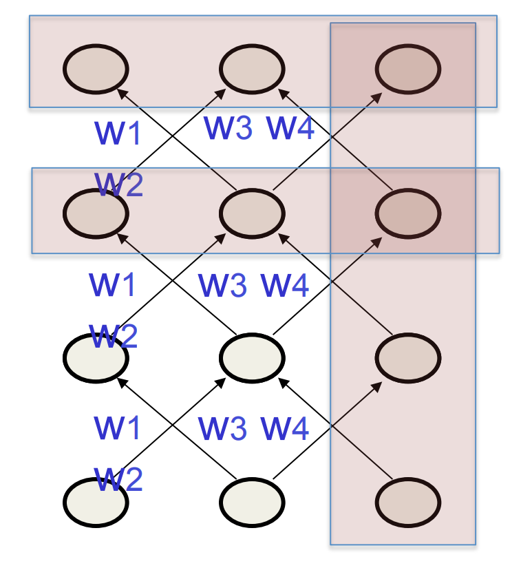
The equivalence between feedforward nets and recurrent nets

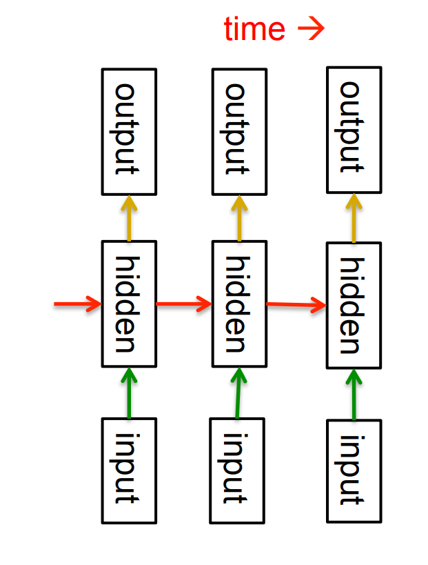
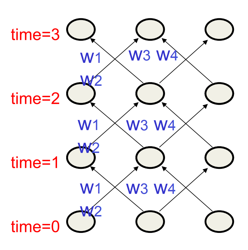
Assume that there is a time delay of 1 in using each connection.

The recurrent net is just a layered net that keeps reusing the same weights.

Reminder: Backpropagation with weight constraints

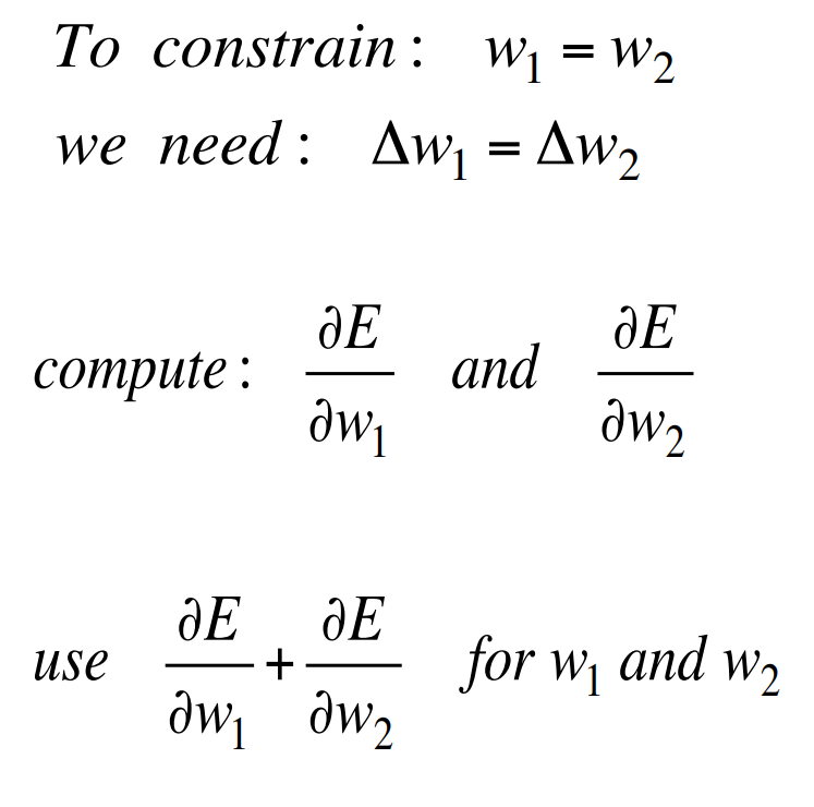
• It is easy to modify the backprop algorithm to incorporate linear constraints between the weights.
• We compute the gradients as usual, and then modify the gradients so that they satisfy the constraints.
  • So if the weights started off satisfying the constraints, they will continue to satisfy them.

Backpropagation through time

• We can think of the recurrent net as a layered, feed-forward net with shared weights and then train the feed-forward net with weight constraints.
• We can also think of this training algorithm in the time domain:
  • The forward pass builds up a stack of the activities of all the units at each time step.
  • The backward pass peels activities off the stack to compute the error derivatives at each time step.
  • After the backward pass we add together the derivatives at all the different times for each weight.

An irritating extra issue

• We need to specify the initial activity state of all the hidden and output units.
• We could just fix these initial states to have some default value like 0.5.
• But it is better to treat the initial states as learned parameters.
• We learn them in the same way as we learn the weights.
  • Start off with an initial random guess for the initial states.
  • At the end of each training sequence, backpropagate through time all the way to the initial states to get the gradient of the error function with respect to each initial state.
  • Adjust the initial states by following the negative gradient.

Providing input to recurrent networks

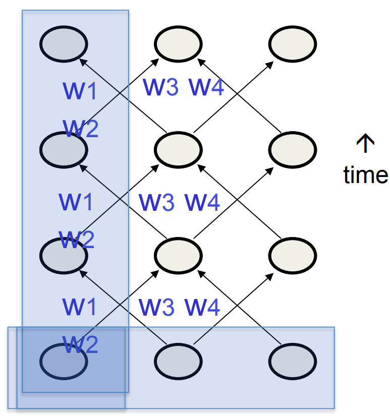
• We can specify inputs in several ways:
  • Specify the initial states of all the units.
  • Specify the initial states of a subset of the units.
  • Specify the states of the same subset of the units at every time step.
• This is the natural way to model most sequential data.

Teaching signals for recurrent networks

• We can specify targets in several ways:
  • Specify desired final activities of all the units
  • Specify desired activities of all units for the last few steps
• Good for learning attractors
• It is easy to add in extra error derivatives as we backpropagate.
  • Specify the desired activity of a subset of the units.
• The other units are input or hidden units.