Deep Neural Networks - Notes for lecture 6e

Lecture 6e: Rmsprop: Divide the gradient by a running average of its recent magnitude

some learning rate algorithms

This is another method that treats every weight separately. rprop uses the method of video 6d, plus that it only looks at the sign of the gradient.

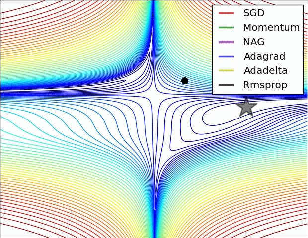
Make sure to understand how momentum🚀 is like using a (weighted) average of past gradients.

Synonyms: “moving average”, “running average”, “decaying average”.

All of these describe the same method of getting a weighted average of past observations, where recent observations are weighted more heavily than older ones.

That method is shown in video 6e at 5:04. (there, it’s a running average of the square of the gradient)

“moving average” and “running average” are fairly generic. “running average” is the most commonly used phrase.

“decaying average” emphasizes the method that’s used to compute it: there’s a decay factor in there, like the alpha in the momentum🚀 method.

rprop: Using only the sign of the gradient

• The magnitude of the gradient can be very different for different weights and can change during learning.
  • This makes it hard to choose a single global learning rate.
• For full batch learning, we can deal with this variation by only using the sign of the gradient.
  • The weight updates are all of the same magnitude.
  • This escapes from plateaus with tiny gradients quickly.
    
• rprop: This combines the idea of only using the sign of the gradient with the idea of adapting the step size separately for each weight.
  • Increase the step size for a weight multiplicatively (e.g. times 1.2) if the signs of its last two gradients agree.
  • Otherwise decrease the step size multiplicatively (e.g. times 0.5).
  • Limit the step sizes to be less than 50 and more than a millionth (Mike Shuster’s advice).

Why rprop does not work with mini-batches

• The idea behind stochastic gradient descent is that when the learning rate is small, it averages the gradients over successive minibatches.
  • Consider a weight that gets a gradient of +0.1 on nine minibatches and a gradient of -0.9 on the tenth mini-batch.
    
  • We want this weight to stay roughly where it is.
• rprop would increment the weight nine times and decrement it once by about the same amount (assuming any adaptation of the step sizes is small on this time-scale).
  • So the weight would grow a lot.
• Is there a way to combine:
  • The robustness of rprop.
  • The efficiency of mini-batches.
  • The effective averaging of gradients over mini-batches.

rmsprop: A mini-batch version of rprop

• rprop is equivalent to using the gradient but also dividing by the size of the gradient.
  • The problem with mini-batch rprop is that we divide by a different number for each mini-batch. So why not force the number we divide by to be very similar for adjacent mini-batches?
    
• rmsprop Keep a moving average of the squared gradient for each weight

MeanSquare(w,t) = 0.9 \times MeanSquare(w, t−1) \times 0.1 \bigg(\frac{∂E}{∂w}(t)\bigg)^2 - Dividing the gradient by \sqrt{MeanSquare(w, t)} makes the learning work much better (Tijmen Tieleman, unpublished).

Further developments of rmsprop

• Combining rmsprop with standard momentum🚀
  • Momentum does not help as much as it normally does. Needs more investigation.
• Combining rmsprop with Nesterov momentum🚀 (Sutskever 2012) [elshamy2023improving]
  • It works best if the RMS of the recent gradients is used to divide the correction rather than the jump in the direction of accumulated corrections.
• Combining rmsprop with adaptive learning rates for each connection
  • Needs more investigation.
• Other methods related to rmsprop
  • Yann LeCun’s group has a fancy version in (Schaul, Zhang, and LeCun 2013)

Summary of learning methods for neural networks

• For small datasets (e.g. 10,000 cases) or bigger datasets without much redundancy, use a full-batch method.
  • Conjugate gradient, LBFGS …
  • adaptive learning rates, rprop …
• For big, redundant datasets use minibatches.
  • Try gradient descent with momentum. 🚀
  • Try rmsprop (with momentum🚀 ?)
  • Try LeCun’s latest recipe.
• Why there is no simple recipe:
  • Neural nets differ a lot:
    • Very deep nets (especially ones with narrow bottlenecks).
    • Recurrent nets.
      
    • Wide shallow nets. -Tasks differ a lot:
    • Some require very accurate weights, some don’t.
    • Some have many very rare cases (e.g. words).

References

Schaul, Tom, Sixin Zhang, and Yann LeCun. 2013. “No More Pesky Learning Rates.” https://arxiv.org/abs/1206.1106.