Deep Neural Networks - Notes for lecture 6d

Lecture 6d: Adaptive learning rates for each connection

This is really “for each parameter”, i.e. biases as well as connection strengths. Vocabulary: a “gain” is a multiplier. This video introduces a basic idea (see the video title), with a simple implementation. In the next video, we’ll see a more sophisticated implementation. You might get the impression from this video that the details of how best to use such methods are not universally agreed on. That’s true. It’s research in progress.

The intuition behind separate adaptive learning rates

• In a multilayer net, the appropriate learning rates can vary widely between weights:
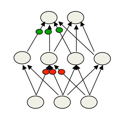
  • The magnitudes of the gradients are often very different for different layers, especially if the initial weights are small.
  • The fan-in of a unit determines the size of the “overshoot” effects caused by simultaneously changing many of the incoming weights of a unit to correct the same error.
• So use a global learning rate (set by hand) multiplied by an appropriate local gain that is determined empirically for each weight.

Gradients can get very small in the early layers of very deep nets.

The fan-in often varies widely between layers.

One way to determine the individual learning rates

• Start with a local gain of 1 for every weight.
  
• Increase the local gain if the gradient for that weight does not change sign.
• Use small additive increases and multiplicative decreases (for mini-batch)
  • This ensures that big gains decay rapidly when oscillations start.
  • If the gradient is totally random the gain will hover around 1 when we increase by plus \delta half the time and decrease by times 1-\delta half the time.

\Delta w_{ij} = -\epsilon g_{ij} \frac{∂E}{∂_{w_{ij}}} \text{if } (\frac{∂E}{∂_{w_{ij}}}(t)\frac{∂E}{∂_{w_{ij}}}(t-1))>0 \text{then } g_{ij}(t) = g_{ij}(t − 1) + .05

\text{else } g_{ij}(t) = g_{ij} δ (t − 1 ) \times .95

Tricks for making adaptive learning rates work better

• Limit the gains to lie in some reasonable range
  • e.g. [0.1, 10] or [.01, 100]
• Use full batch learning or big minibatches
  • This ensures that changes in the sign of the gradient are not mainly due to the sampling error of a minibatch.
• Adaptive learning rates can be combined with momentum.
  • Use the agreement in sign between the current gradient for a weight and the velocity for that weight (Jacobs, 1989).
    
• Adaptive learning rates only deal with axis-aligned effects.
  • Momentum 🚀 does not care about the alignment of the axes.