Deep Neural Networks - Notes for lecture 6c

Lecture 6c: The momentum method

Drill down into momentum mentioned before.
The biggest challenge in this video is to think of the error surface as a mountain landscape. If you can do that, and you understand the analogy well, this video will be easy. You may have to go back to video 3b, which introduces the error surface. Important concepts in this analogy: “ravine”, “a low point on the surface”, “oscillations”, “reaching a low altitude”, “rolling ball”, “velocity”. All of those have meaning on the “mountain landscape” side of the analogy, as well as on the “neural network learning” side of the analogy. The meaning of “velocity” in the “neural network learning” side of the analogy is the main idea of the momentum method.

Vocabulary: the word “momentum” can be used with three different meanings, so it’s easy to get confused. It can mean the momentum method for neural network learning, i.e. the idea that’s introduced in this video. This is the most appropriate meaning of the word. It can mean the viscosity constant (typically 0.9), sometimes called alpha, which is used to reduce the velocity. It can mean the velocity. This is not a common meaning of the word. Note that one may equivalently choose to include the learning rate in the calculation of the update from the velocity, instead of in the calculation of the velocity.

The intuition behind the momentum method

Momentum intution

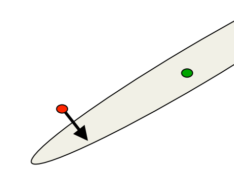
• Imagine a ball on the error surface. The location of the ball in the horizontal plane represents the weight vector.
  • The ball starts off by following the gradient, but once it has velocity, it no longer does steepest descent.
    
  • Its momentum makes it keep going in the previous direction.
• It damps oscillations in directions of high curvature by combining gradients with opposite signs.
• It builds up speed in directions with a gentle but consistent gradient.

The equations of the momentum method

The effect of the gradient is to increment the previous velocity. The velocity also decays by \alpha which is slightly less then 1. v(t) =α v(t −1)−ε \frac{∂E}{∂w}(t)

The weight change is equal to the current velocity.

\begin{align} Δw(t) &= v(t) \\ &= α v(t −1)−ε \frac{∂E}{∂w}(t) \\ &= α Δw(t −1)−ε \frac{∂E}{∂w}(t) \end{align}

The weight change can be expressed in terms of the previous weight change and the current gradient.

The behavior of the momentum method

• If the error surface is a tilted plane, the ball reaches a terminal velocity.
  • If the momentum is close to 1, this is much faster than simple gradient descent.
• At the beginning of learning there may be very large gradients.
  • So it pays to use a small momentum (e.g. 0.5).
  • Once the large gradients have disappeared and the weights are stuck in a ravine the momentum can be smoothly raised to its final value (e.g. 0.9 or even 0.99)
• This allows us to learn at a rate that would cause divergent oscillations without the momentum.

v(∞) = \frac{1}{1−α} \biggr( −ε \frac{∂E}{∂w} \biggr)

A better type of momentum (Nesterov 1983)

• The standard momentum method first computes the gradient at the current location and then takes a big jump in the direction of the updated accumulated gradient.
• Ilya Sutskever (2012 unpublished) suggested a new form of momentum that often works better.
  • Inspired by the Nesterov method for optimizing convex functions.
    
• First make a big jump in the direction of the previous accumulated gradient.
• Then measure the gradient where you end up and make a correction.
  • Its better to correct a mistake after you have made it!

A picture of the Nesterov method

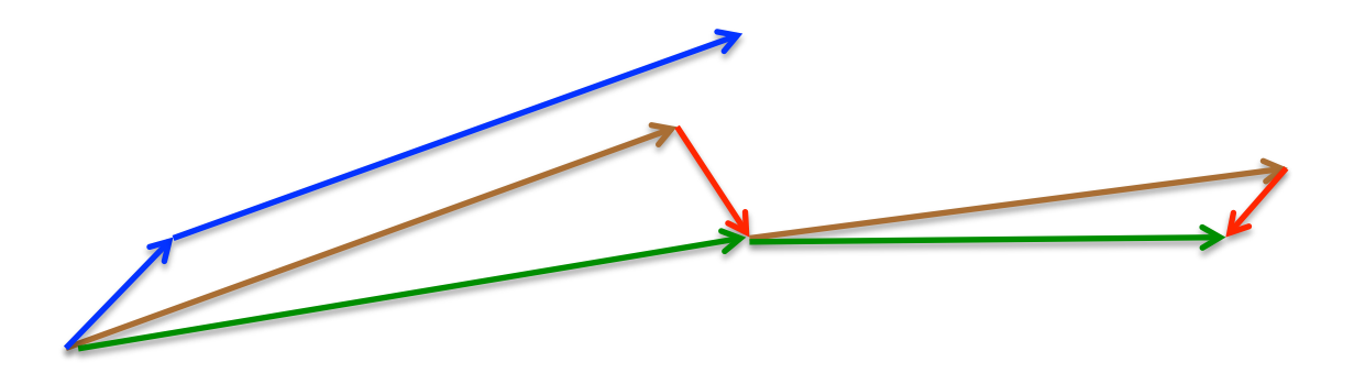
brown vector = jump,
red vector = correction,
green vector = accumulated gradient blue vectors = standard momentum

• First make a big jump in the direction of the previous accumulated gradient.
• Then measure the gradient where you end up and make a correction.