Deep Neural Networks - Notes for lecture 6b

Lecture 6b: A bag of tricks for mini-batch gradient descent

initializing weights: we must not initialize units with equal weights as they can never become different. we cannot use zero as it will remain zero we want to avoid explosion and vanishing weights fan in - the number of inputs
Part 1 is about transforming the data to make learning easier. At 1:10, there’s a comment about random weights and scaling. The “it” in that comment is the average size of the input to the unit. At 1:15, the “good principle”: what he means is INVERSELY proportional. At 4:38, Geoff says that the hyperbolic tangent is twice the logistic minus one. This is not true, but it’s almost true. As an exercise, find out’s missing in that equation. At 5:08, Geoffrey suggests that with a hyperbolic tangent unit, it’s more difficult to sweep things under the rug than with a logistic unit. I don’t understand his comment, so if you don’t either, don’t worry. This comment is not essential in this course: we’re never using hyperbolic tangents in this course. Part 2 is about changing the stochastic gradient descent algorithm in sophisticated ways. We’ll look into these four methods in more detail, later on in the course. Jargon: “stochastic gradient descent” is mini-batch or online gradient descent. The term emphasizes that it’s not full-batch gradient descent. “stochastic” means that it involves randomness. However, this algorithm typically does not involve randomness. However, it would be truly stochastic if we would randomly pick 100 training cases from the entire training set, every time we need the next mini-batch. We call traditional “stochastic gradient descent” stochastic because it is, in effect, very similar to that truly stochastic version. Jargon: a “running average” is a weighted average over the recent past, where the most recent past is weighted most heavily.

Be careful about turning down the learning rate

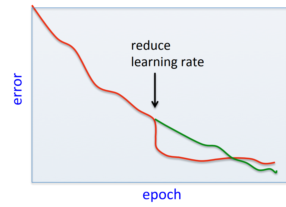
• Turning down the learning rate reduces the random fluctuations in the error due to the different gradients on different mini-batches. -So we get a quick win.
  • But then we get slower learning.
• Don’t turn down the learning rate too soon!

Initializing the weights

• If two hidden units have exactly the same bias and exactly the same incoming and outgoing weights, they will always get exactly the same gradient.
  • So they can never learn to be different features.
  • We break symmetry by initializing the weights to have small random values.
• If a hidden unit has a big fan-in, small changes on many of its incoming weights can cause the learning to overshoot.
  • We generally want smaller incoming weights when the fan-in is big, so initialize the weights to be proportional to sqrt(fan-in).
• We can also scale the learning rate the same way.

Shifting the inputs

Shifting the inputs

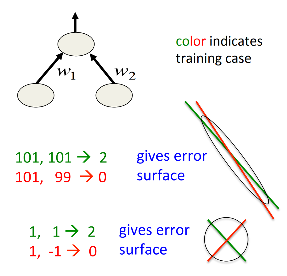
• When using steepest descent, shifting the input values makes a big difference. -It usually helps to transform each component of the input vector so that it has zero mean over the whole training set.
  
• The hypberbolic tangent (which is 2*logistic -1) produces hidden activations that are roughly zero mean.
  -In this respect its beYer than the logistic.

Scaling the inputs

Scaling the inputs

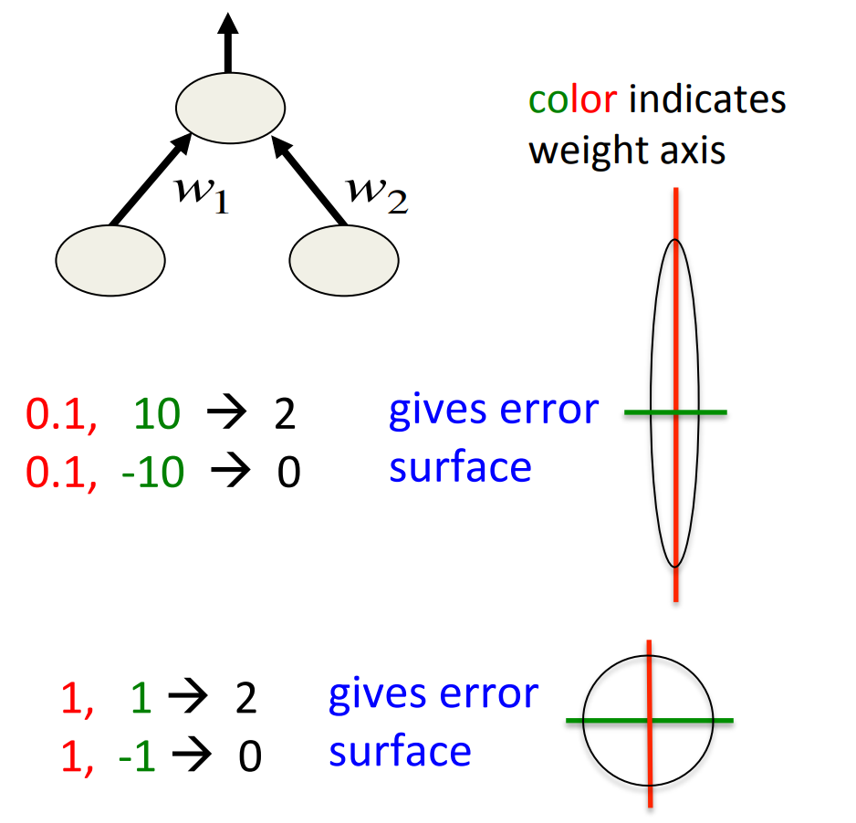
• When using steepest descent, scaling the input values makes a big difference.
  • It usually helps to transform each component of the input vector so that it has unit variance over the whole training set.

A more thorough method: Decorrelate the input components

• For a linear neuron, we get a big win by decorrelating each component of the input from the other input components.
• There are several different ways to decorrelate inputs. A reasonable method is to use Principal Components Analysis.
  • Drop the principal components with the smallest eigenvalues.
    • This achieves some dimensionality reduction.
  • Divide the remaining principal components by the square roots of their eigenvalues. For a linear neuron, this converts an axis aligned elliptical error surface into a circular one.
• For a circular error surface, the gradient points straight towards the minimum.

Common problems that occur in multilayer networks

• If we start with a very big learning rate, the weights of each hidden unit will all become very big and positive or very big and negative.
  • The error derivatives for the hidden units will all become tiny and the error will not decrease.
  • This is usually a plateau, but people often mistake it for a local minimum.
• In classification networks that use a squared error or a cross-entropy error, the best guessing strategy is to make each output unit always produce an output equal to the proportion of time it should be a 1.
  • The network finds this strategy quickly and may take a long time to improve on it by making use of the input.
    
  • This is another plateau that looks like a local minimum.

Four ways to speed up mini-batch learning

• Use “momentum”
  • Instead of using the gradient to change the position of the weight “particle”, use it to change the velocity.
    
• Use separate adaptive learning rates for each parameter
  • Slowly adjust the rate using the consistency of the gradient for that parameter.
• rmsprop: Divide the learning rate for a weight by a running average of the magnitudes of recent gradients for that weight.
  • This is the mini-batch version of just using the sign of the gradient.
    
• Take a fancy method from the optimization literature that makes use of curvature information (not this lecture)
  • Adapt it to work for neural nets
  • Adapt it to work for mini-batches.