slides for the lesson
Why is a new algorithm needed?
- The Perceptron learning procedure cannot be generalized to more layers because for those the mean of two good solutions may not be a good set of weights.
- Before we showed that we were approximating better sets of weights in this algorithm we want to improve the output as a response of the input.
- Motivation: We want to use this to learn prices.
- Our strategy is to reduce overall error, unlike with a perceptron we cannot guarantee we will get better individual estimates.
Lecture 3a: Learning the weights of a linear neuron
lecure video
A different way to show that a learning procedure makes progress
- Instead of showing the weights get closer to a good set of weights, show that the actual output values get closer the target values.
- This can be true even for non-convex problems in which there are many quite different sets of weights that work well and averaging two good sets of weights may give a bad set of weights.
- It is not true for perceptron learning.
- The simplest example is a linear neuron with a squared error measure.
Linear neurons
- Called linear filters in electrical engineering and linear transforms in linear algebra and can be represented by martracies
- We don’t use linear neurons in practice:
- Without a non-linearity in the unit, a stack of N layers can be replaced by a single layer 2
- This lecture just demonstrates the analysis we will use with non-linear units.
- The neuron’s output is the real valued weighted sum of its inputs
- The goal of learning is to minimize the total error over all training cases.
- Here error is the squared difference between the desired output and the actual output.
\textcolor{green}{\overbrace{y}^{\text{output}}} = \sum_{n \in train} \textcolor{red}{\overbrace{w_i}^{\text{weights}}} \textcolor{blue}{\underbrace{x_i}_{\text{inputs}}}= \vec{w}^T\cdot\vec{x} where:
- y is the neuron’s estimate of the desired output
- x is the input vector
- w is the weight vector
Why don’t we solve it analytically?
- It is straight-forward to write down a set of equations, one per training case, and to solve for the best set of weights.
- This is the standard engineering approach so why don’t we use it?
- Scientific answer: We want a method that real neurons could use.
- Engineering answer: We want a method that can be generalized to multi-layer, non-linear neural networks.
- The analytic solution relies on it being linear and having a squared error measure.
- Iterative methods are usually less efficient but they are much easier to generalize.
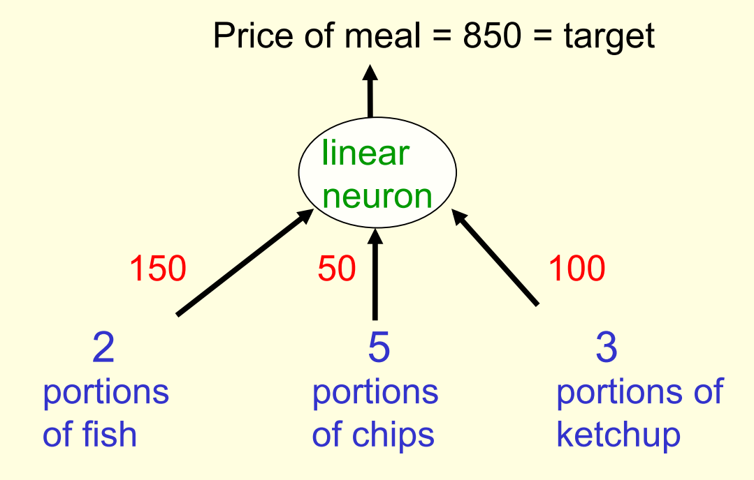
A toy example
- Each day you get lunch at the cafeteria.
- Your diet consists of fish, chips, and ketchup.
- You get several portions of each.
- The cashier only tells you the total price of the meal
- After several days, you should be able to figure out the price of each portion.
- The iterative approach: Start with random guesses for the prices and then adjust them to get a better fit to the observed prices of whole meals.
Solving the equations iteratively
- Each meal price gives a linear constraint on the prices of the portions:
\text{price} = X_\text{fish} W_\text{fish} + X_\text{chips} W_\text{chips} + X_\text{ketchup}W_\text{ketchup}
- The prices of the portions are like the weights in of a linear neuron. W = (w_\text{fish} , W_\text{ chips} , W_\text{ketchup} )
- We will start with guesses for the weights and then adjust the guesses slightly to give a better fit to the prices given by the cashier.
The true weights used by the cashier
- We will start with guesses for the weights and then adjust the guesses slightly to give a better fit to the prices given by the cashier.
A model of the cashier with arbitrary initial weights

- Residual error = 350
- The “delta-rule” for learning is: \Delta w_i = \epsilon x_i (t - y)
- With a learning rate \epsilon of 1/35, the weight changes are:+20, +50, +30
- This gives new weights of: 70, 100, 80.
- The weight for chips got worse, but over all the weights are better
y reducing errors, individual weight estimate may be getting worse
Calculating the change in the weights:
calculate our output using forward propagation
Deriving the delta rule
y = \sum_{n \in train} w_i x_i= \vec{w}^T\vec{x} Define the error as the squared residuals summed over all training cases:
E = \frac{1}{2}\sum_{n \in train} (t_n−y_n)^2
use the chain rule to get error derivatives for weights
\frac{d E}{\partial w_i}=\frac{1}{2}\sum_{n \in train}\frac{\partial y^n}{\partial w_i} \frac{dE}{dy^n}=\frac{1}{2}\sum_{n \in train}x_i^n(t^n−y^n)
the batch delta rule changes the weight in proportion to their error derivative summed on all training cases times the learning rate
\Delta w_i = −\epsilon \frac{d E}{\partial w_i} = \sum_{n \in train} \epsilon x_i^n (t^n−y^n)
Behaviour of the iterative learning procedure
- Does the learning procedure eventually get the right answer?
- There may be no perfect answer.
- By making the learning rate small enough we can get as close as we desire to the best answer.
- How quickly do the weights converge to their correct values?
- It can be very slow if two input dimensions are highly correlated. If you almost always have the same number of portions of ketchup and chips, it is hard to decide how to divide the price between ketchup and chips
The relationship between the online delta-rule and the learning rule for perceptrons
- In perceptron learning, we increment or decrement the weight vector by the input vector.
- But we only change the weights when we make an error.
- In the online version of the delta-rule we increment or decrement the weight vector by the input vector scaled by the residual error and the learning rate.
- So we have to choose a learning rate. This is annoying
- residual error
- it’s the amount by which we got the answer wrong.
A very central concept is introduced without being made very explicit: we use derivatives for learning, i.e. for making the weights better. Try to understand why those concepts are indeed very related.
- on-line learning
- means that we change the weights after every training example that we see, and we typically cycle through the collection of available training examples.
Lecture 3b: The error surface for a linear neuron

- The error surface lies in a space with a horizontal axis for each weight and one vertical axis for the error.
- For a linear neuron with a squared error, it is a quadratic bowl.
- Vertical cross-sections are parabolas.
- Horizontal cross-sections are ellipses.
- For multi-layer, non-linear nets the error surface is much more complicated.
Online versus batch learning

Why learning can be slow

- If the ellipse is very elongated, the direction of steepest descent is almost perpendicular to the direction towards the minimum!
- The red gradient vector has a large component along the short axis of the ellipse and a small component along the long axis of the ellipse.
- This is just the opposite of what we want.
Lecture 3c: Learning the weights of a logistic output neuron
Logistic neurons AKA linear filters - useful to understand the algorithm but in reality we need to use non linear activation function.
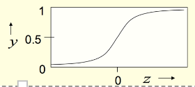
Logistic neurons
These give a real-valued output that is a smooth and bounded function of their total input. They have nice derivatives which make learning easy.
z = b + \sum _i x_i w_i
y=\frac{1}{1+e^{-z}}
The derivatives of a logistic neuron
The derivatives of the logit, z, with respect to the inputs and the weights are very simple:
z = b + \sum _i x_i w_i \tag{the logit}
\frac{\partial z}{\partial w_i} = x_i \;\;\;\;\; \frac{\partial z}{\partial x_i} = w_i
The derivative of the output with respect to the logit is simple if you express it in terms of the output:
y=\frac{1}{1+e^{-z}}
\frac{d y}{d z} = y( 1-y)
since
y = \frac{1}{1+e^{-z}}=(1+e^{-z})^{-1} differentiating \frac{d y}{d z} = \frac{-1(-e^{-z})}{(1+e^{-z})^2} =\frac{1}{1+e^{-z}} \frac{e^{-z}}{1+e^{-z}} = y( 1-y) Using the chain rule to get the derivatives needed for learning the weights of a logistic unit To learn the weights we need the derivative of the output with respect to each weight:
\frac{d y}{\partial w_i} =\frac{\partial z}{\partial w_i} \frac{dy}{dz} = x_iy( 1-y)
\frac{d E}{\partial w_i} = \frac{\partial y^n}{\partial w_i} \frac{dE}{dy^n} = - \sum \green{x_i^n}\red{ y^n( 1-y^n)}\green{(t^n-y^n)}
where the green part corresponds to the delta rule and the extra term in red is simply the slope of the logistic.
The error function is still:
E =\frac{1}{2}(y−t)^2
Notice how after Hinton explained what the derivative is for a logistic unit, he considers the job to be done. That’s because the learning rule is always simply some learning rate multiplied by the derivative.
Lecture 3d: The back-propagation algorithm
Here, we start using hidden layers. To train them, we need the back propagation algorithm. Hidden layers, and this algorithm, are very important. They are the layers between the input layer and the output.
The story of training by perturbations also makes an appearance in the course by David MCcay, serving primarily as motivation for the back propagation algorithm.
This computation, just like the forward propagation, can be vectorized across multiple units in every layer, and multiple training cases.
Learning by perturbing weights
- Randomly perturb one weight and see if it improves performance. If so, save the change.
- This is a form of reinforcement learning.
- Very inefficient. We need to do multiple forward passes on a representative set of training cases just to change one weight. Back propagation is much better.
- Towards the end of learning, large weight perturbations will nearly always make things worse, because the weights need to have the right relative values. (so we should adapt a decreasing learning rate).
- We could randomly perturb all the weights in parallel and correlate the performance gain with the weight changes.
- Not any better because we need lots of trials on each training case to “see” the effect of changing one weight through the noise created by all the changes to other weights.
- A better idea: Randomly perturb the activities of the hidden units.
- Once we know how we want a hidden activity to change on a given training case, we can compute how to change the weights.
- There are fewer activities than weights, but backpropagation still wins by a factor of the number of neurons.
The idea behind backpropagation
- We don’t know what the hidden units ought to do, but we can compute how fast the error changes as we change a hidden activity.
- Instead of using desired activities to train the hidden units, use error derivatives w.r.t. hidden activities.
- Each hidden activity can affect many output units and can therefore have many separate effects on the error. These effects must be combined.
- Instead of using desired activities to train the hidden units, use error derivatives w.r.t. hidden activities.
- We can compute error derivatives for all the hidden units efficiently at the same time.
- Once we have the error derivatives for the hidden activities, its easy to get the error derivatives for the weights going into a hidden unit.
Sketch of back propagation on a single case
- First convert the discrepancy between each output and its target value into an error derivative.
- Then compute error derivatives in each hidden layer from error derivatives in the layer above.
- Then use error derivatives w.r.t. activities to get error derivatives w.r.t. the incoming weights. E =\frac{1}{2}(t_i-y_i)^2
\frac{\partial E}{\partial y_j}=-(t_j-y_j)


Lecture 3e: Using the derivatives computed by backpropagation
The backpropagation algorithm is an efficient way of computing the error derivative \frac{dE}{dw} for every weight on a single training case. There are many decisions needed on how to derive new weights using there derivatives.
- Optimization issues: How do we use the error derivatives on individual cases to discover a good set of weights? (lecture 6)
- Generalization issues: How do we ensure that the learned weights work well for cases we did not see during training? (lecture 7)
We now have a very brief overview of these two sets of issues.
How often to update weights ?
- Online - after every case.
- Mini Batch - after a small sample of training cases.
- Full Batch - after a full sweep of training data.
How much to update? (c.f. lecture 6)
- fixed learning rate
- adaptable global learning rate
- adaptable learning rate per weight
- don’t use steepest descent (velocity/momentum/second order methods)
Overfitting: The downside of using powerful models
Regularization- How to ensure that learned weights work well for cases we did not see during training?
- The training data contains information about the regularities in the mapping from input to output. But it also contains two types of noise.
- The target values may be unreliable (usually only a minor worry).
- There is
sampling error. There will be accidental regularities just because of the particular training cases that were chosen.
- When we fit the model, it cannot tell which regularities are real and which are caused by sampling error.
- So it fits both kinds of regularity.
- If the model is very flexible it can model the sampling error really well. This is a disaster.
A simple example of overfitting

- Which output value should you predict for this test input?
- Which model do you trust?
- The complicated model fits the data better.
- But it is not economical.
- A model is convincing when it fits a lot of data surprisingly well.
- It is not surprising that a complicated model can fit a small amount of data well.
- Models fit both signal and noise.
How to reduce overfitting
- A large number of different methods have been developed to reduce overfitting.
- Weight-decay
- Weight-sharing - reduce model flexibility by adding constraints on weights
- Early stopping - stop training when by monitoring the Test error.
- Model averaging - use an ensemble of models
- Bayesian fitting of neural nets - like averaging but weighed
- Dropout - (hide data from half the net)
- Generative pre-training - (more data)
- Many of these methods will be described in lecture 7.
Footnotes
Reuse
Citation
@online{bochman2017,
  author = {Bochman, Oren},
  title = {Deep {Neural} {Networks} - {Notes} for {Lesson} 3},
  date = {2017-08-01},
  url = {https://orenbochman.github.io/notes/dnn/dnn-03/l_03.html},
  langid = {en}
}