Deep Neural Networks - Notes for lecture 3c

Lecture 3c: Learning the weights of a logistic output neuron

Logistic neurons AKA linear filters - useful to understand the algorithm but in reality we need to use non linear activation function.

Logistic neurons

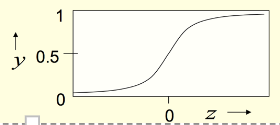
These give a real-valued output that is a smooth and bounded function of their total input. They have nice derivatives which make learning easy.

z = b + \sum _i x_i w_i

y=\frac{1}{1+e^{-z}}

logistic activation function

The derivatives of a logistic neuron

The derivatives of the logit, z, with respect to the inputs and the weights are very simple:

z = b + \sum _i x_i w_i \tag{the logit}

\frac{\partial z}{\partial w_i} = x_i \;\;\;\;\; \frac{\partial z}{\partial x_i} = w_i

The derivative of the output with respect to the logit is simple if you express it in terms of the output:

y=\frac{1}{1+e^{-z}}

\frac{d y}{d z} = y( 1-y)

since

y = \frac{1}{1+e^{-z}}=(1+e^{-z})^{-1} differentiating \frac{d y}{d z} = \frac{-1(-e^{-z})}{(1+e^{-z})^2} =\frac{1}{1+e^{-z}} \frac{e^{-z}}{1+e^{-z}} = y( 1-y) Using the chain rule to get the derivatives needed for learning the weights of a logistic unit To learn the weights we need the derivative of the output with respect to each weight:

\frac{d y}{\partial w_i} =\frac{\partial z}{\partial w_i} \frac{dy}{dz} = x_iy( 1-y)

\frac{d E}{\partial w_i} = \frac{\partial y^n}{\partial w_i} \frac{dE}{dy^n} = - \sum {\color{green}{x_i^n}}{\color{red}{ y^n( 1-y^n)}}{\color{green}{(t^n-y^n)}}

where the green part corresponds to the delta rule and the extra term in red is simply the slope of the logistic.

The error function is still:

E =\frac{1}{2}(y−t)^2

Notice how after Hinton explained what the derivative is for a logistic unit, he considers the job to be done. That’s because the learning rule is always simply some learning rate multiplied by the derivative.