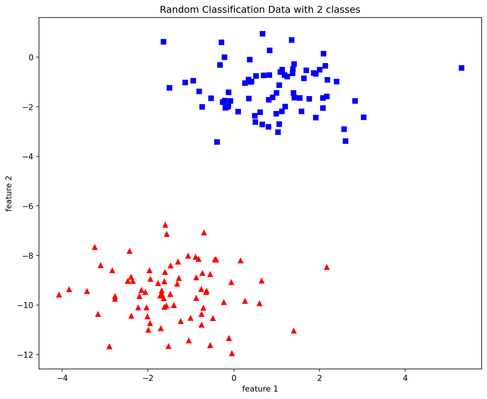
Deep Neural Networks - Notes for lecture 2b

The lecture starts with the history of Perceptrons (Wikipedia contributors 2024)

Then covers with The perceptron convergence procedure. Next is a deeper dive into the computational geometry of Perceptrons

I also added a python implementation from scratch.

Lecture 2b: Perceptrons: The first generation of neural networks

The standard paradigm for statistical pattern recognition

The standard Perceptron architecture

1. Convert the raw input vector into a vector of feature activations. Use hand-written programs based on common-sense to define the features.
2. Learn how to weight each of the feature activations to get a single scalar quantity.
3. If this quantity is above some threshold, decide that the input vector is a positive example of the target class.

The history of Perceptrons

• Perceptrons were introduced in (Rosenblatt 1962) by Frank Rosenblatt who popularized them
  • They appeared to have a very powerful learning algorithm.
  • Lots of grand claims were made for what they could learn to do.
• In (Minsky and Papert 1969) the authors, analysed what Perceptrons could do and showed their limitations. ¹
  • Many people thought these limitations applied to all neural network models.
• The perceptron learning procedure is still widely used today for tasks with enormous feature vectors that contain many millions of features.

A perceptron

• why the bias can be implemented as a special input unit?
• biases can be treated using weights using an input that is always one.
• a threshold is equivalent to having a negative bias.
• we can avoid having to figure out a separate learning rule for the bias by using a trick:
• A bias is exactly equivalent to a weight on an extra input line that always has an activation of 1.

Binary threshold neurons (decision units)

Binary Theshold Unit

• Introduced in (Mcculloch and Pitts 1943)
  • First compute a weighted sum of the inputs from other neurons (plus a bias).
  • Then output a 1 if the weighted sum exceeds zero.

z = b+ \sum_i{ x_i w_i} y = \left\{ \begin{array}{ll} 1 & \text{if} \space z \ge 0 \\ 0 & \text{otherwise} \end{array} \right.

How to learn biases using the same rule as we use for learning weights

• A threshold is equivalent to having a negative bias.
• We can avoid having to figure out a separate learning rule for the bias by using a trick:
  • A bias is exactly equivalent to a weight on an extra input line that always has an activity of 1.
  • We can now learn a bias as if it were a weight.

The Perceptron convergence procedure: Training binary output neurons as classifiers

• Add an extra component with value 1 to each input vector. The bias weight on this component is minus the threshold. Now we can forget the threshold.
• Pick training cases using any policy that ensures that every training case will keep getting picked.
  • If the output unit is correct, leave its weights alone.
  • If the output unit incorrectly outputs a zero, add the input vector to the weight vector.
  • If the output unit incorrectly outputs a 1, subtract the input vector from the weight vector.
• This is guaranteed to find a set of weights that gets the right answer for all the training cases if any such set exists.

A full implementation of a perceptrons:

code and image from: Implementing the Perceptron Algorithm in Python

Perceptron

from sklearn import datasets
from matplotlib import pyplot as plt
import numpy as np

X, y = datasets.make_blobs(n_samples=150,n_features=2,
                           centers=2,cluster_std=1.05,
                           random_state=2)
#Plotting
fig = plt.figure(figsize=(10,8))
plt.plot(X[:, 0][y == 0], X[:, 1][y == 0], 'r^')
plt.plot(X[:, 0][y == 1], X[:, 1][y == 1], 'bs')
plt.xlabel("feature 1")
plt.ylabel("feature 2")
plt.title('Random Classification Data with 2 classes')

def step_func(z):
        return 1.0 if (z > 0) else 0.0
      
def perceptron(X, y, lr, epochs):
    '''
    X: inputs
    y: labels
    lr: learning rate
    epochs: Number of iterations
    m: number of training examples
    n: number of features 
    '''
    m, n = X.shape    
    # Initializing parapeters(theta) to zeros.
    # +1 in n+1 for the bias term.
    theta = np.zeros((n+1,1))
    
    # list with misclassification count per iteration.
    n_miss_list = []
    
    # Training.
    for epoch in range(epochs):
        # variable to store misclassified.
        n_miss = 0
        # looping for every example.
        for idx, x_i in enumerate(X):
            # Inserting 1 for bias, X0 = 1.
            x_i = np.insert(x_i, 0, 1).reshape(-1,1)          
            # Calculating prediction/hypothesis.
            y_hat = step_func(np.dot(x_i.T, theta))
            # Updating if the example is misclassified.
            if (np.squeeze(y_hat) - y[idx]) != 0:
                theta += lr*((y[idx] - y_hat)*x_i)
                # Incrementing by 1.
                n_miss += 1
        # Appending number of misclassified examples
        # at every iteration.
        n_miss_list.append(n_miss)
    return theta, n_miss_list

Text(0.5, 0, 'feature 1')

Text(0, 0.5, 'feature 2')

Text(0.5, 1.0, 'Random Classification Data with 2 classes')

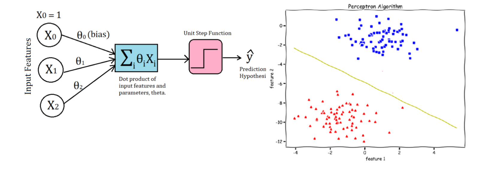
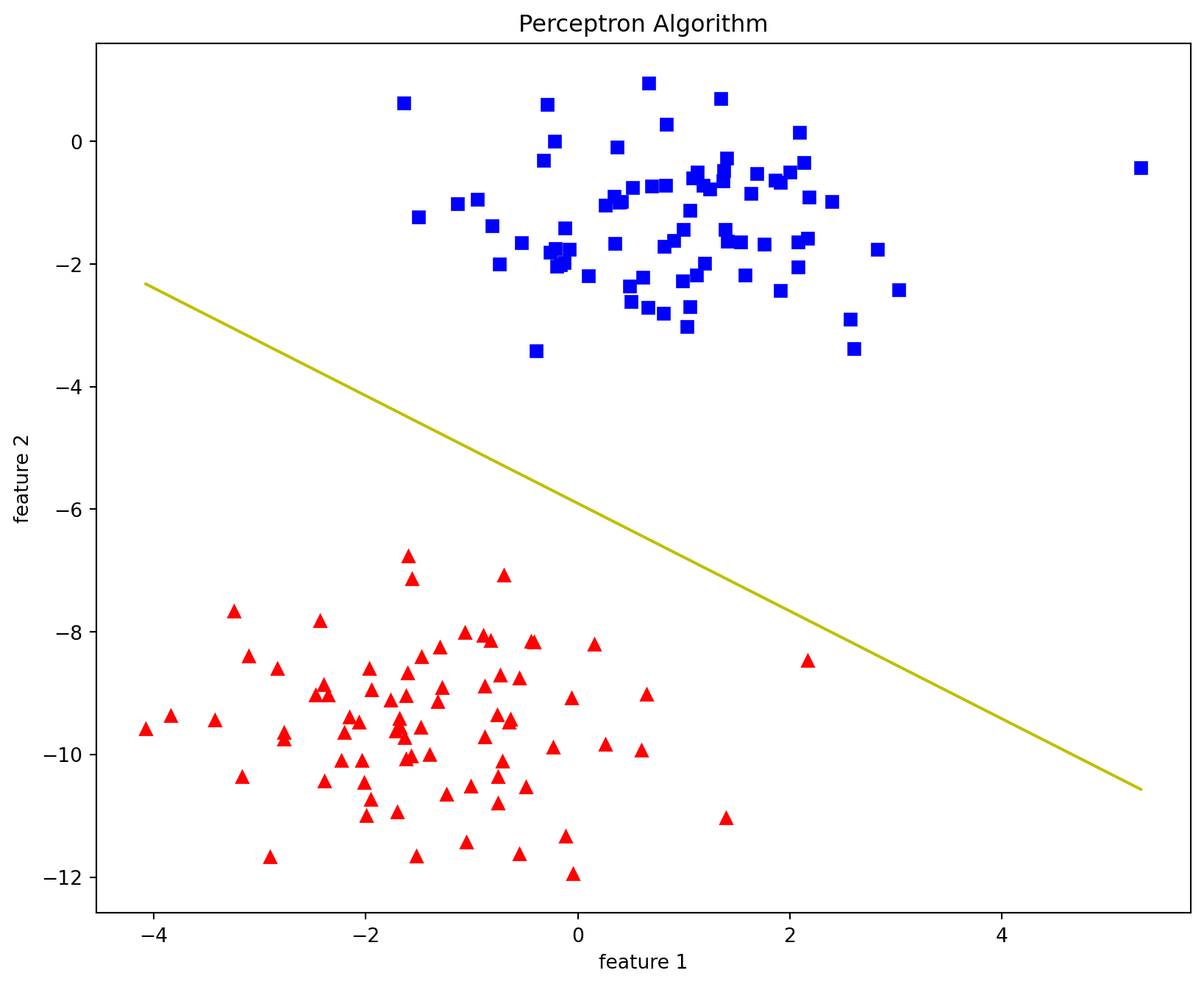
def plot_decision_boundary(X, theta):
    
    # X --> Inputs
    # theta --> parameters
    
    # The Line is y=mx+c
    # So, Equate mx+c = theta0.X0 + theta1.X1 + theta2.X2
    # Solving we find m and c
    x1 = [min(X[:,0]), max(X[:,0])]
    m = -theta[1]/theta[2]
    c = -theta[0]/theta[2]
    x2 = m*x1 + c
    
    # Plotting
    fig = plt.figure(figsize=(10,8))
    plt.plot(X[:, 0][y==0], X[:, 1][y==0], "r^")
    plt.plot(X[:, 0][y==1], X[:, 1][y==1], "bs")
    plt.xlabel("feature 1")
    plt.ylabel("feature 2")
    plt.title('Perceptron Algorithm')
    plt.plot(x1, x2, 'y-')

theta, miss_l = perceptron(X, y, 0.5, 100)
plot_decision_boundary(X, theta)

References

Mcculloch, Warren, and Walter Pitts. 1943. “A Logical Calculus of Ideas Immanent in Nervous Activity.” Bulletin of Mathematical Biophysics 5: 127–47.

Minsky, Marvin, and Seymour Papert. 1969. Perceptrons: An Introduction to Computational Geometry. Cambridge, MA, USA: MIT Press.

Rosenblatt, F. 1962. Principles of Neurodynamics: Perceptrons and the Theory of Brain Mechanisms. Cornell Aeronautical Laboratory. Report No. VG-1196-g-8. Spartan Books. https://www.google.com/books?id=7FhRAAAAMAAJ.

Wikipedia contributors. 2024. “Perceptron — Wikipedia, the Free Encyclopedia.” https://en.wikipedia.org/w/index.php?title=Perceptron&oldid=1195848318.

Footnotes

1. The main results are available here