
Week1: Logistic Regression
It’s possible to do sentiment analysis in a much simpler way than shown in this course. Logistic regression isn’t as simple as OLS regrsion due to having categorical features. Finally Stochastic Gradient Descent isn’t the standard way of solving logistic regression, Maximum Likelihood Estimation is. I think they use SGD so it’s more familiar later in the specialization. However if we want to flatten our learning curve consider the following videos which will help us get more confident with logistic regression by building from the more familiar OLS regression.
| video | subject |
|---|---|
| StatQuest: Logistic Regression | |
| Logistic Regression Details Pt1: Coefficients | |
| Logistic Regression Details Pt 2: Maximum Likelihood |
Supervised ML & Sentiment Analysis
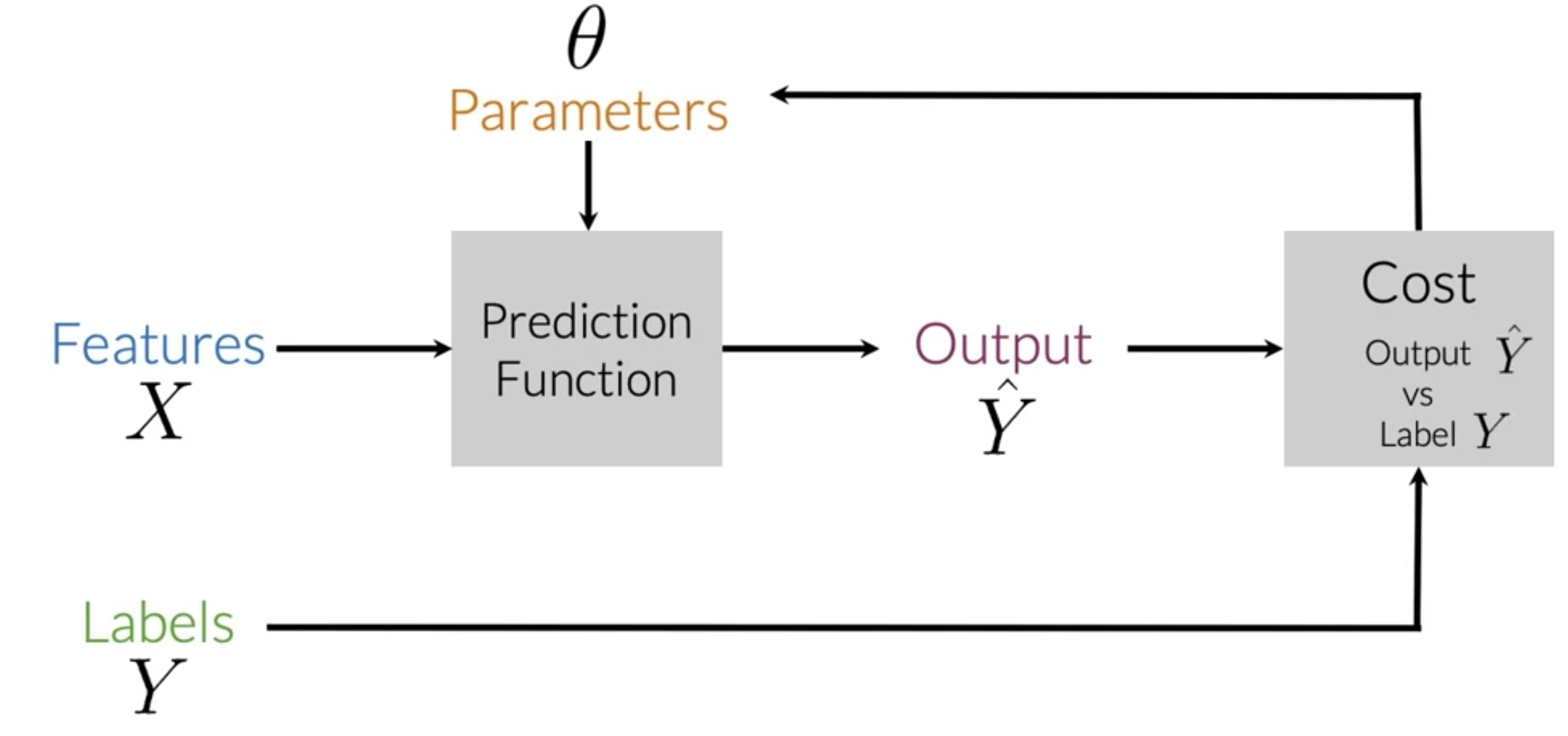
- In supervised ML we get a dataframe with input features X and their corresponding ground truth label Y.
- The goal is to minimize prediction error rates, AKA cost.
- To do this, one runs the prediction function which takes in parameters and map the features of an input to an output label \hat{Y}.
- The optimal mapping from features to labels is when the difference between the expected values Y and the predicted values \hat{Y} is minimized.
- The cost function F does this by comparing how closely the output \hat{Y} is to the label Y.
- Update the parameters and repeat the whole process until the cost is minimized.
- We use the sigmoid cost function:
Sentiment Analysis
If we are passionate about NLP here is a gem to get we started. This is a popular science with many ideas for additional classifiers using pronouns.
| video | subject |
|---|---|
| The Secret Life of Pronouns: James Pennebaker at TEDxAustin | |
| Language of Truth and Lies: I-words | |
| LIWC-22 2022 Tutorial 1: Getting started with LIWC-22 | |
| Likelihood |
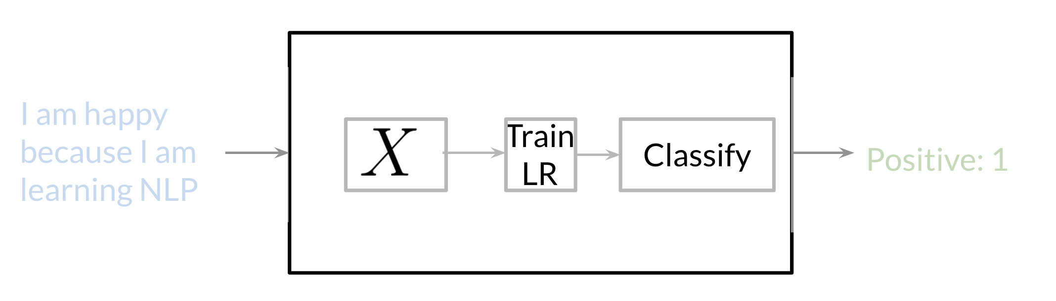
Supervised ML & Sentiment Analysis
- One example of a Supervised machine learning classification task for
sentiment analysis - The objective is to predict whether a tweet has a positive or negative sentiment. (If it is positive/optimistic or negative/pessimistic).
To perform sentiment analysis on a tweet, we need to:
- represent the text for example “I am happy because I am learning NLP” as features,
- train a logistic regression classifier
- 1 for a positive sentiment
- 0 for negative sentiment.
- and then we use it to classify the text.
Vocabulary & Feature Extraction
Sparse Representation
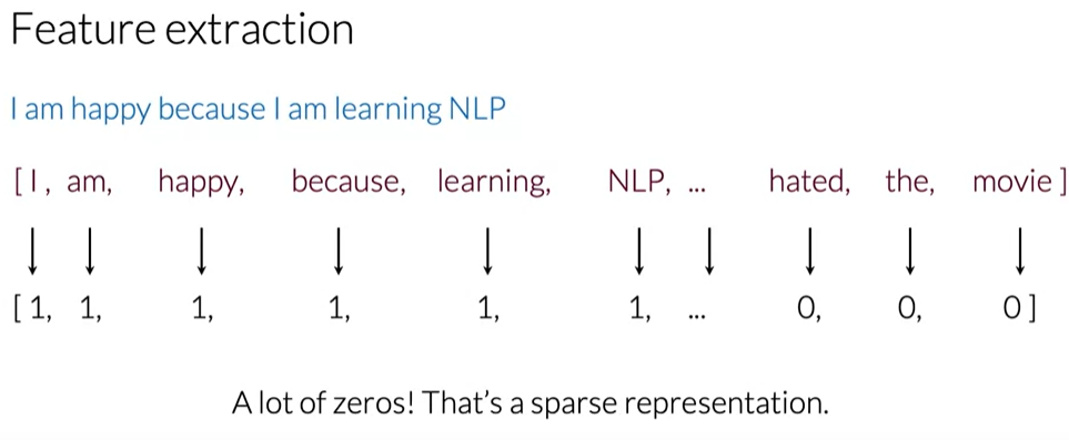
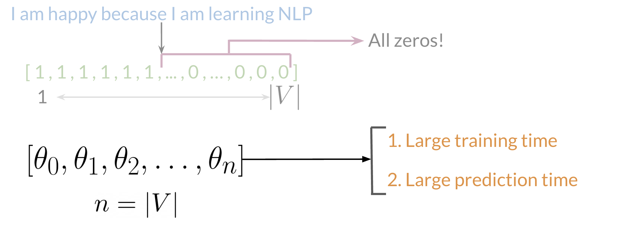
Given a tweet, or some text, one can represent it as a vector. The vector has a dimension |V|, where V corresponds to the size of the vocabulary size. If we had the tweet “I am happy because I am learning NLP,” then we would put a 1 in the corresponding index for any word in the tweet, and a 0 otherwise.
As V gets larger, the vector becomes more sparse. Furthermore, we end up having many more features and end up training \theta_0 \ldots \theta_n parameters. This results in a larger training time. And the inference time increases as well.
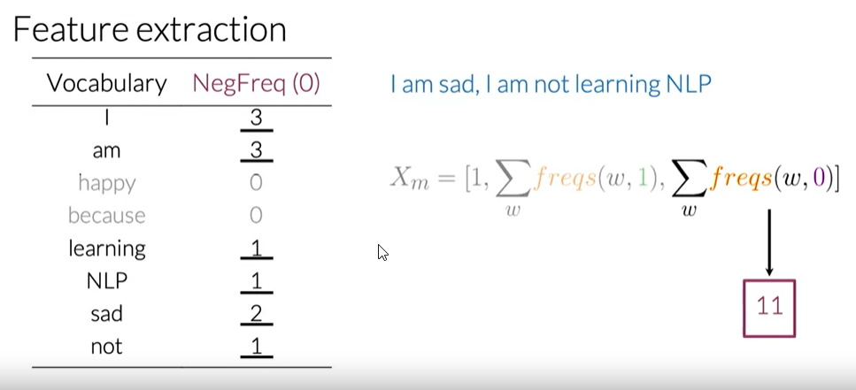
Feature Extraction based on class frequencies
| Positive tweets | Negative tweets |
|---|---|
| I am happy because I am learning NLP | I am sad, I am not learning NLP |
| I am happy | I am sad |
Given a corpus with positive and negative tweets we can represent it as follows:
| Vocabulary | PosFreq (1) | NegFreq (O) |
|---|---|---|
| I | 3 | 3 |
| am | 3 | 3 |
| happy | 2 | 0 |
| because | 1 | 0 |
| learning | 1 | 1 |
| NLP | 1 | 1 |
| sad | 0 | 2 |
| not | 0 | 1 |
freqs: dictionary mapping from (word, class) to frequency :
\underbrace{X_m}_{\textcolor{#7200ac}{\text{Features of tweet M}}} =\left[ \underbrace{1}_{\textcolor{#126ed5}{\text{bias}}} ,\sum_w \underbrace{\textcolor{#da7801}{freqs}(w,\textcolor{#2db15d}{1})}_{\textcolor{#931e18}{\text{Sum Pos.frequencies}}} ,\sum_w \underbrace{\textcolor{#da7801}{freqs}(w,\textcolor{#931e18}{0})}_{\textcolor{#2db15d}{\text{Sum Neg. frequencies}}} \right]
we have to encode each tweet as a vector. Previously, this vector was of dimension VV. Now, as we’ll see in the upcoming videos, we’ll represent it with a vector of dimension 33. We create a dictionary to map the word, it class, either positive or negative, to the number of times that word appeared in its corresponding class.
Preprocessing
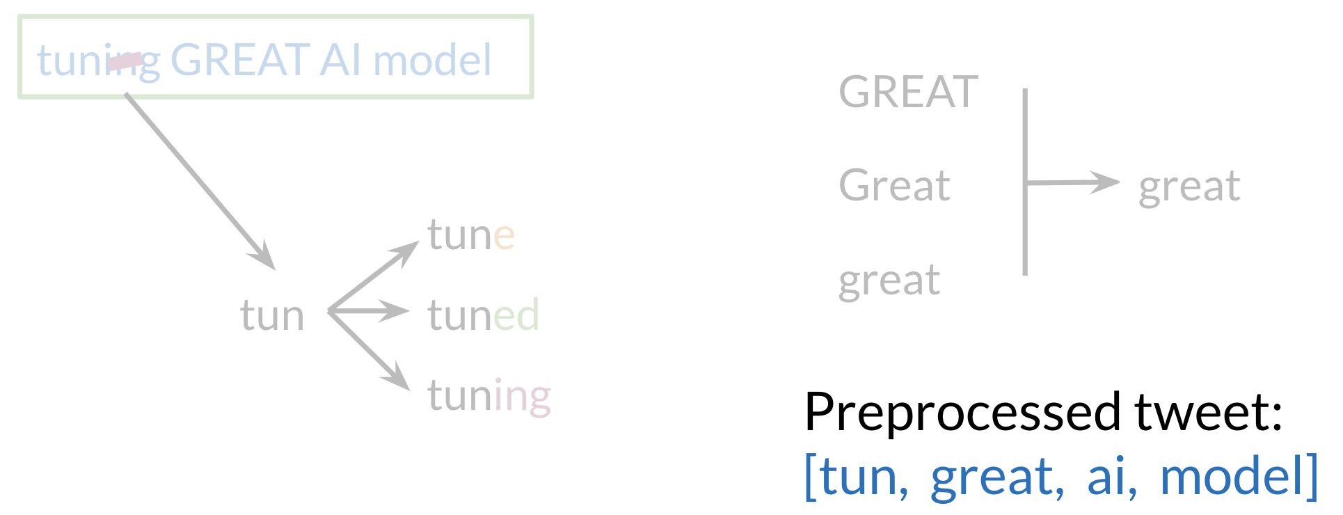
When preprocessing, we have to perform the following:
- Eliminate handles and URLs
- Tokenize the string into words.
- Remove stop words like “and, is, a, on, etc.”
- Stemming - converting each word to its stem. For example dancer, dancing, danced, becomes ‘danc’. We can use porter’s stemmer to take care of this.
- Convert all our words to lower case.
Training Logistic Regression
{}
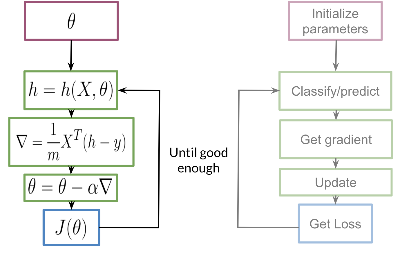
To train our logistic regression function, we’ll do the following: we initialize our parameter \theta , that we can use in you sigmoid, we then compute the gradient that we’ll use to update , and then calculate the cost. we keep doing so until good enough
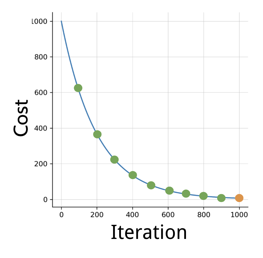
Usually we keep training until the cost converges. If we were to plot the number of iterations versus the cost, we should see something like this:
Testing Logistic Regression

To test our model, we would run a subset of our data, known as the validation set, on our model to get predictions. The predictions are the outputs of the sigmoid function. If the output is ≥=0.5, we would assign it to a positive class. Otherwise, we would assign it to a negative class. To compute accuracy, we solve the following equation:
accuracy = \sum \frac{pred^{(i)}==y^{(i)}_{val}}{m}
Cross validation note:
- In reality, given your X data we would usually split it into three components. X{train}, X{val}, X{test}.
- The distribution usually varies depending on the size of our data set. However, a 80%, 10%, 10% split usually works.
In other words, we go over all our training examples, m of them, and then for every prediction, if it was wright we add a one. we then divide by m.
Logistic Regression: Cost Function
We should start by developing intuition about how the cost function is designed the way it is. This is important because we’ll meet the sigmoid in Neural Networks, job interviews and so best make a friend of it. In(Hinton 2012) there is the full derivation of Sigmoid cost function. Also the sigmoid and Logistic regression are intimately related - we can’t have one without the other.
In plain english: “The cost function is mean log loss across all training examples”
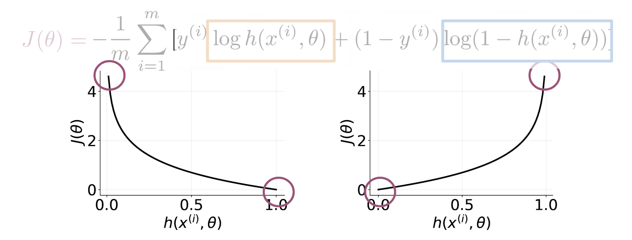
J( \theta)=−\frac{1}{m} \sum^m_{i=1}[y^{(i)}\log h(x^{(i)}, \theta)+(1 −y^{(i)}) \log (1−h(x^{(i)}, \theta))]
where:
- m is the count of rows of our training set.
- i indexes a single row in the dataset.
- x^{(i)} is the data for row i.
- y^{(i)} is the
gound truthAKAlabelfor rows i. - h(x^{(i)},\theta) is the model’s prediction for row ith row.
We’ll derive the logistic regression cost function to get the gradients.
we can see in the figure:
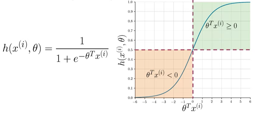
- If y = 1 and our prediction is close to 0, we get a cost close to ∞.
- The same applies when y=0 and we predict ion is close to 1.
- On the other hand if we get a prediction equal to the label, we get a cost of 0.
- In either, case we are trying to minimize J(\theta)
Mathematical Derivation
To see why the cost function is designed that way, let’s take a step back and write up a function that compresses the two cases into one case. If
P(y|x(i), \theta) =h(x^{(i)}, \theta)^{y^{(i)}}1−h(x^{(i)}, \theta)^{1−y^{(i)}}
From the preceding, we can see that when y = 1, we get h(x^{(i)}, \theta)^{y^{(i)}} and when y≈0 we ther term 1 − h(x^{(i)}, \theta)^{(1−y^{(i)})}, which makes sense, since the two probabilities equal to 1. In either case, we want to maximize the function $ h(x^{(i)}, )^{y(i)}$ by making it as close to 1 as possible.
When y ≈ 0 , we want the term 1-h(x^{(i)}, \theta)^{1−y^{(i)}} ≈ 0 which then \implies h(x^{(i)}, \theta)^{y^{(i)}} ≈ 1 When y=1, we want h(x^{(i)}, \theta)^{y^{(i)}} = 1 Now we want to find a way to model the entire data set and not just one example. To do so, we’ll define the likelihood as follows:
L(\theta) = \prod^m_{i=1} h(\theta, x^{(i)})^{y^{(i)}} (1−h(\theta, x^{(i)}))^{(1−y^{(i)})}
Note that if we mess up the classification of one example, we end up messing up the overall likelihood score, which is exactly what we intended. We want to fit a model to the entire dataset where all data points are related. to
\lim_{m \to \infty} L(\theta) = 0
It goes close to zero, because both h(\theta, x^{(i)})^{y^{(i)}} and (1−h(\theta, x^{(i)}))^{(1−y^{(i)})} are bounded by [0,1]. Since we are trying to maximize h(\theta, x^{(i)}) in L(\theta), we can introduce the log and just maximize the log of the function.
Introducing the log, allows us to write the log of a product as the sum of each log. Here are two identities that will come in handy:
\log(a*b*c) = \log(a) + \log(b) + \log(c)
and
\log(a^b) = b \times \log(a)
Given the two preceding identities, we can rewrite the equation as follows: \begin{align*} \max_{ h(x^{(i)},\theta)}\log L(\theta) &= \log \prod^m_{i=1}h(x^{(i)}, \theta)^{y^{(i)}}(1−h(x^{(i)} ,\theta))^{1−y^{(i)}} \\ &= \sum^m_{i=1} \log h(x^{(i)}, \theta)^{y^{(i)}} (1−h(x^{(i)}, \theta)^{1−y^{(i)}}) \\ &= \sum^m_{i=1} \log h(x^{(i)}, \theta)^{y^{(i)}} + \log(1−h(x^{(i)}, \theta)^{1−y^{(i)}} \\ &= \sum^m_{i=1} y^{(i)}\log h(x^{(i)}, \theta) + (1−y^{(i)}) \log(1−h(x^{(i)}, \theta)) \end{align*} Hence, we now divide by m, because we want to see the average cost. \begin{align*} \frac{1}{m} \sum^m_{i=1} y^{(i)}\log h(x^{(i)}, \theta) + (1−y^{(i)}) \log(1−h(x^{(i)}, \theta)) \end{align*}
Remember that we were maximizing h(\theta, x(i)) in the preceding equation. It turns out that maximizing an equation is the same as minimizing its negative. Think of x^2, feel free to plot it to see that for we yourself. Hence we add a negative sign and we end up minimizing the cost function as follows.
\begin{align*} J(\theta)= − \frac{1}{m} \sum^m_{i=1} [y^{(i)} \log h(x^{(i)}, \theta) + ( 1 − y^{(i)}) \log ( 1 − h(x^{(i)}, \theta))] \end{align*}
A vectorized implementation is:
\begin{align*} & h = g(X\theta)\newline & J(\theta) = \frac{1}{m} \cdot \left(-y^{T}\log(h)-(1-y)^{T}\log(1-h)\right) \end{align*}
Logistic Regression: Gradient
\mathbf{w}(t+1) = \mathbf{w}(t) - \eta\nabla E_{in}
For the case of logistic regression, the gradient of the error measure with respect to the weights, is calculated as:
\nabla E_{in}\left(\mathbf{w}\right) = -\frac{1}{N}\sum\limits_{n=1}^N \frac{y_n\mathbf{x_N}}{1 + \exp\left(y_n \mathbf{w^T}(t)\mathbf{x_n}\right)}
Let’s look into the gradient descent in more detail, as the gradient update rule is given without an explicitly derivation.
The general form Of gradient descent is defined
\begin{align*} & Repeat \; \lbrace \newline & \; \theta_j := \theta_j - \alpha \dfrac{\partial}{\partial \theta_j}J(\theta) \newline & \rbrace \end{align*}
We can work out the derivative part using Calculus to get:
\begin{align*} & Repeat \; \lbrace \theta_j := \theta_j - \frac{\alpha}{m} \sum_{i=1}^m ( h(x^{(i)}, \theta) - y^{(i)}) x_j^{(i)} \rbrace \end{align*}
A vectorized formulation \theta_j := \theta_j - \frac{\alpha}{m} X^T ( H(X, \theta) -Y)
Partial derivative of J(\theta)
\begin{align*} h(x)'&=\left(\frac{1}{1+e^{-x}}\right)'=\frac{-(1+e^{-x})'}{(1+e^{-x})^2}=\frac{-1'-(e^{-x})'}{(1+e^{-x})^2}=\frac{0-(-x)'(e^{-x})}{(1+e^{-x})^2}=\frac{-(-1)(e^{-x})}{(1+e^{-x})^2}=\frac{e^{-x}}{(1+e^{-x})^2} \newline &=\left(\frac{1}{1+e^{-x}}\right)\left(\frac{e^{-x}}{1+e^{-x}}\right)=h(x)\left(\frac{+1-1 + e^{-x}}{1+e^{-x}}\right)=h(x)\left(\frac{1 + e^{-x}}{1+e^{-x}} - \frac{1}{1+e^{-x}}\right)=h(x)(1 - h(x)) \end{align*}
\begin{align*} \frac{\partial}{\partial \theta_j} J(\theta) &= \frac{\partial}{\partial \theta_j} \frac{-1}{m}\sum_{i=1}^m \left [ y^{(i)} log ( h(x^{(i)}, \theta) ) + (1-y^{(i)}) log (1 - h(x^{(i)}, \theta)) \right ] \newline &= - \frac{1}{m}\sum_{i=1}^m \left [ y^{(i)} \frac{\partial}{\partial \theta_j} log ( h(x^{(i)}, \theta)) + (1-y^{(i)}) \frac{\partial}{\partial \theta_j} log (1 - h(x^{(i)}, \theta))\right ] \newline &= - \frac{1}{m}\sum_{i=1}^m \left [ \frac{y^{(i)} \frac{\partial}{\partial \theta_j} h(x^{(i)}, \theta)}{ h(x^{(i)}, \theta)} + \frac{(1-y^{(i)})\frac{\partial}{\partial \theta_j} (1 - h(x^{(i)}, \theta))}{1 - h(x^{(i)}, \theta)}\right ] \newline &= - \frac{1}{m}\sum_{i=1}^m \left [ \frac{y^{(i)} \frac{\partial}{\partial \theta_j} h(x^{(i)}, \theta)}{ h(x^{(i)}, \theta)} + \frac{(1-y^{(i)})\frac{\partial}{\partial \theta_j} (1 - h(x^{(i)}, \theta))}{1 - h(x^{(i)}, \theta)}\right ] \newline &= - \frac{1}{m}\sum_{i=1}^m \left [ \frac{y^{(i)} h(x^{(i)}, \theta) (1 - h(x^{(i)}, \theta)) \frac{\partial}{\partial \theta_j} \theta^T x^{(i)}}{ h(x^{(i)}, \theta)} + \frac{- (1-y^{(i)}) h(x^{(i)}, \theta)(1 - h(x^{(i)}, \theta)) \frac{\partial}{\partial \theta_j} \theta^T x^{(i)}}{1 - h(x^{(i)}, \theta)}\right ] \newline &= - \frac{1}{m}\sum_{i=1}^m \left [ \frac{y^{(i)} h(x^{(i)}, \theta) (1 - h(x^{(i)}, \theta)) \frac{\partial}{\partial \theta_j} \theta^T x^{(i)}}{ h(x^{(i)}, \theta)} - \frac{(1-y^{(i)}) h(x^{(i)}, \theta) (1 - h(x^{(i)}, \theta)) \frac{\partial}{\partial \theta_j} \theta^T x^{(i)}}{1 - h(x^{(i)}, \theta)}\right ] \newline &= - \frac{1}{m}\sum_{i=1}^m \left [ y^{(i)} (1 - h(x^{(i)}, \theta)) x^{(i)}_j - (1-y^{(i)}) h(x^{(i)}, \theta) x^{(i)}_j\right ] \newline &= - \frac{1}{m}\sum_{i=1}^m \left [ y^{(i)} (1 - h(x^{(i)}, \theta)) - (1-y^{(i)}) h(x^{(i)}, \theta) \right ] x^{(i)}_j \newline &= - \frac{1}{m}\sum_{i=1}^m \left [ y^{(i)} - y^{(i)} h(x^{(i)}, \theta) - h(x^{(i)}, \theta) + y^{(i)} h(x^{(i)}, \theta) \right ] x^{(i)}_j \newline &= - \frac{1}{m}\sum_{i=1}^m \left [ y^{(i)} - h(x^{(i)}, \theta) \right ] x^{(i)}_j \newline &= \frac{1}{m}\sum_{i=1}^m \left [ h(x^{(i)}, \theta) - y^{(i)} \right ] x^{(i)}_j \end{align*} {#eq-partial-derivative-Of-J(B) }
First calculate derivatüe Of Sigmoid function (it be useful while finding partial derivative Of Note that we computed the partial derivative Of the Sigmoid function If We Were to derive , 9) with respect to O_j, we would get —
Note that used the chain rule there. ’“e multiply by the derivative Of with respect to Now we are ready to find out result.ng partial derivative;
The Vectorized Version:
\nabla J(\theta) = \frac{1}{m} X^T \cdot (H(X,\theta)-Y)
resources:
- derivative of cost function for Logistic Regression Congratulations. we now know the full derivation Of logistic regression.
- An Intuitive Explanation of Bayes’ Theorem
- (Chadha 2020) Aman Chadha’s Notes
- Ibrahim Jelliti’s Notes
References
Reuse
Citation
@online{bochman2020,
  author = {Bochman, Oren},
  title = {Classification \& {Vector} {Spaces} - {Logistic}
    {Regression}},
  date = {2020-10-23},
  url = {https://orenbochman.github.io/notes/deeplearning.ai-nlp-c1/c1l1-logistic-regression.html},
  langid = {en}
}