Week 2: The AR(p) process

Time Series Analysis

The AR(1) process, Stationarity, ACF, PACF, Differencing, and Smoothing
Coursera
notes
Bayesian Statistics
Autoregressive Models
Time Series
Author

Oren Bochman

Published

Thursday, October 24, 2024

Keywords

time series, stability, order of an AR process, characteristic lag polynomial, autocorrelation function, ACF, partial autocorrelation function, PACF, smoothing, State Space Model, ARMA process, ARIMA, moving average, AR(p) process, R code

Learning Objectives

  • Define the autoregressive process of order p or AR(p) and use R to obtain samples from such process
  • Define ARIMA (autoregressive moving average) models (honors)
  • Perform posterior inference for the AR(p) under the conditional likelihood and the reference prior
  • Perform a full data analysis in R using an AR(p) including
  • likelihood estimation and
  • Bayesian inference,
  • model order selection, and
  • forecasting
  • Explain the relationship between the AR characteristic polynomial, the ACF, the forecast function and the spectral density in the case of an AR(p)

The general AR(p) process (video)

Definition and state-space representation (video)

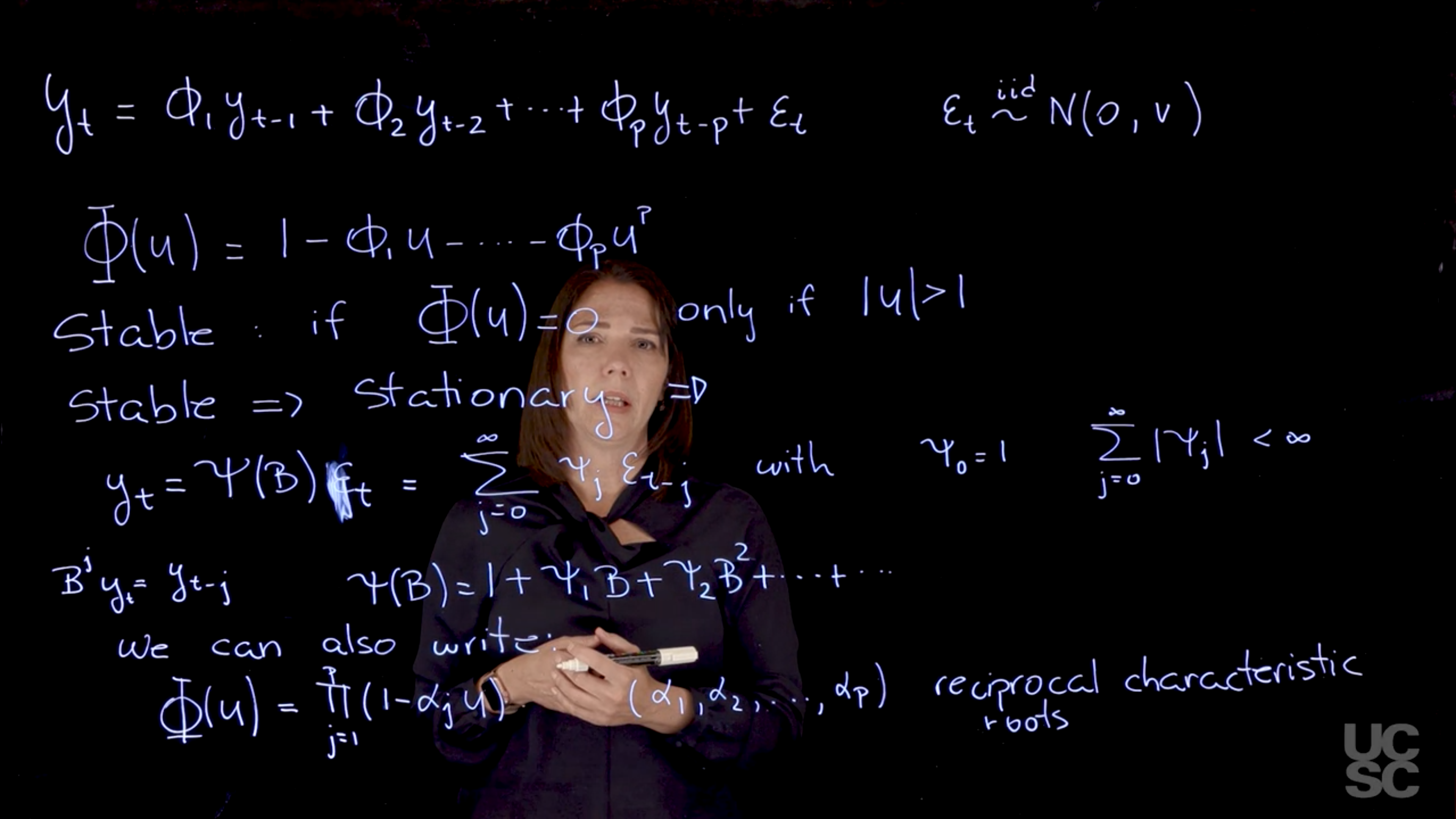
AR(p) process, characteristic polynomial, stability, stationarity and MA representation

AR(p) process, characteristic polynomial, stability, stationarity and MA representation

AR(P) is shorthand for autoregressive process of order p which generalizes the AR(1) process that we studied in the previous module. It is essentially a mapping that allows us to specify the current value of the time series in terms its past p-values and some noise. The number of parameter p, required is the order of the autoregressive process. It tells us how many lags we will be considering.

order

AR(P)

We will assume AR(P) has the following structure:

\textcolor{red}{y_t} = \textcolor{blue}{\phi_1} \textcolor{red}{y_{t-1}} + \textcolor{blue}{\phi_2} \textcolor{red}{y_{t-2}} + \ldots + \textcolor{blue}{\phi_p} \textcolor{red}{y_{t-p}} + \textcolor{grey}{\epsilon_t} \qquad \tag{1}

where:

  • \textcolor{red}{y_t} is the value of the time series at time t

  • \textcolor{blue}{\phi_{1:p}} are the AR coefficients

  • \textcolor{grey}{\epsilon_t} \overset{\text{iid}}{\sim} \text{N}(0,v) \quad \forall t is a white noise process.

  • The number of parameters has increased from one coefficient in AR(1) to p coefficients for AR(P).

A central outcome of the autoregressive nature of the AR(p) is due to the properties the AR characteristic polynomial \Phi. This is defined as :

\Phi AR characteristic polynomial

recall the backshift operator B is defined as B y_t = y_{t-1}, so that B^j y_t = y_{t-j}.

\begin{aligned} y_t &= \phi_1 y_{t-1} + \phi_2 y_{t-2} + \ldots + \phi_p y_{t-p} + \epsilon_t && \text{(Ar(p) defn.)} \newline y_t &= \phi_1 By_{t} + \phi_2 B^2y_{t} + \ldots + \phi_p B^p y_{t} + \epsilon_t && \text{(B defn.)} \newline \epsilon_t &= y_t - \phi_1 B y_t + \phi_2 B^2 y_t + \ldots + \phi_p B^p y_t && \text{(rearranging)} \newline \epsilon_t &= (1- \phi_1 B + \phi_2 B^2 + \ldots + \phi_p B^p) y_t && \text{(factoring out $y_t$)} \end{aligned} \Phi(z) = 1 - \phi_1 z - \phi_2 z^2 - \ldots - \phi_p z^p \qquad \text{(Characteristic polynomial)} \tag{2}

where:

  • z \in \mathbb{C} i.e. complex-valued.

we can also rewrite the characteristic polynomial in terms of the reciprocal roots of the polynomial.

The zeros of the characteristic polynomial are the roots of the AR(p) process.

\Phi(z) = \prod_{j=1}^{p} (1 - \alpha_j z) = 0 \implies z = \frac{1}{ \alpha_j} \qquad \text{(reciprocal roots)}

where:

  • \alpha_j are the reciprocal roots of the characteristic polynomial.

Why are we interested in this autoregresive lag polynomial?

  • This polynomial and its roots informs us a lot about the process and its properties.
  • One of the main characteristics is it allows us to think about things like quasi-periodic behavior, whether it’s present or not in a particular AR(p) process.
  • It allows us to think about whether a process is stationary or not, depending on some properties related to this polynomial.
  • In particular, we are going to say that the process is stable if all the roots of the characteristic polynomial have a modulus greater than one. \Phi(z) = 0 \iff |z| > 1 \qquad \text{(stability condition)} \tag{3}
  • For any of the roots, it has to be the case that the modulus of that root, they have to be all outside the unit circle.
  • If a process is stable, it will also be stationary.
stability condition

We can show this as follows:

  • Once the process is stationary, and if all the roots of the characteristic polynomial are outside the unit circle, then we will be able to write this process in terms of an infinite order moving average process. In this case, if the process is stable, then we are going to be able to write it like this.

y_t = \Psi(B) \epsilon_t = \sum_{j=0}^{\infty} \psi_j \epsilon_{t-j} \ \text {with} \ \psi_0 = 1 \text{ and } \sum_{j=0}^{\infty} |\psi_j| < \infty \tag{4}

where:

  • \epsilon_t is a white noise process with zero mean and constant variance v.
  • B is the lag operator AKA the backshift operator defined by B \varepsilon_t = \varepsilon_{t-1}. This need to be applied to a time series \epsilon_t to get the lagged values.
  • \Psi(B) is the infinite order polynomial in B that representing a linear filter applied to the noise process.​
  • \psi_t = 1 is the weight for the white noise at time t.
  • the constraint \psi_0 = 1 ensures that the current shock contributes directly to y_t
  • the constraint on the weights \sum_{j=0}^{\infty} |\psi_j| < \infty ensures that the weights decay sufficiently fast, so that the process does not explode i.e. it is stable and thus stationary.

the notation with \psi a functional of operator B and \psi_i as constants is confusing in both the reuse if the symbol and the complexity.

Here, U is any complex valued number.

I am going to have an infinite order polynomial here on B, the backshift operator that I can write down just as the sum, j goes from zero to infinity.

Here \psi_0=1. Then there is another condition on the Psi’s for this to happen. We have to have finite sum of these on these coefficients. Once again, if the process is stable, then it would be stationary and we will be able to write down the AR as an infinite order moving average process here. If you recall, B is the backshift operator. Again, if I apply this to y_t, I’m just going to get y_t-j. I can write down Psi of B, as 1 + \psi_1 B, B squared, and so on. It’s an infinite order process.

The AR characteristic polynomial can also be written in terms of the reciprocal roots of the polynomial. So instead of considering the roots, we can consider the reciprocal roots. In that case, let’s say the $phi$ of u for Alpha 1, Alpha 2, and so on. The reciprocal roots. Why do we care about all these roots? Why do we care about this structure? Again, we will be able to understand some properties of the process based on these roots as we will see.

A state space representation of Ar(p)

A state space representation of Ar(p)

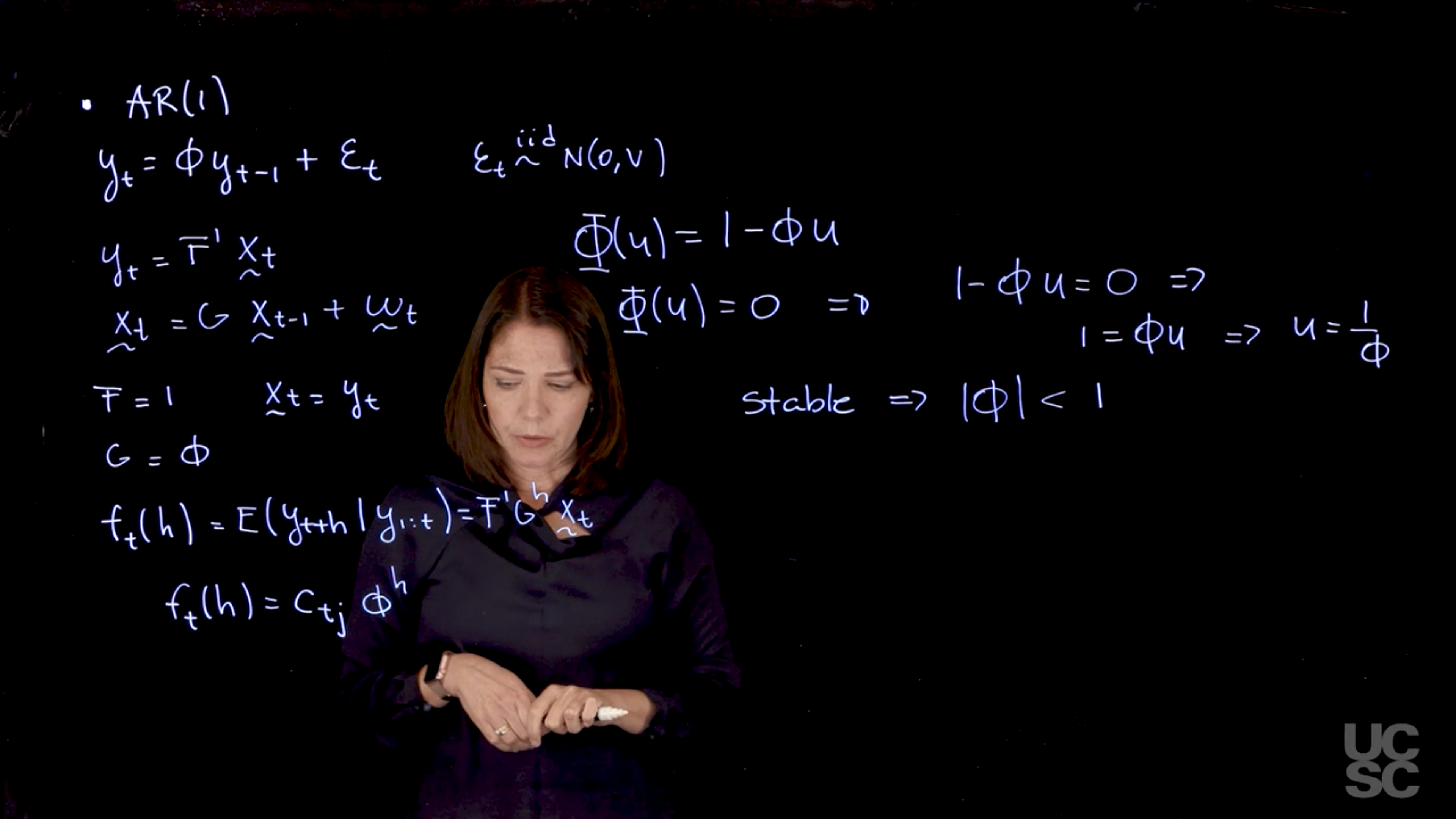
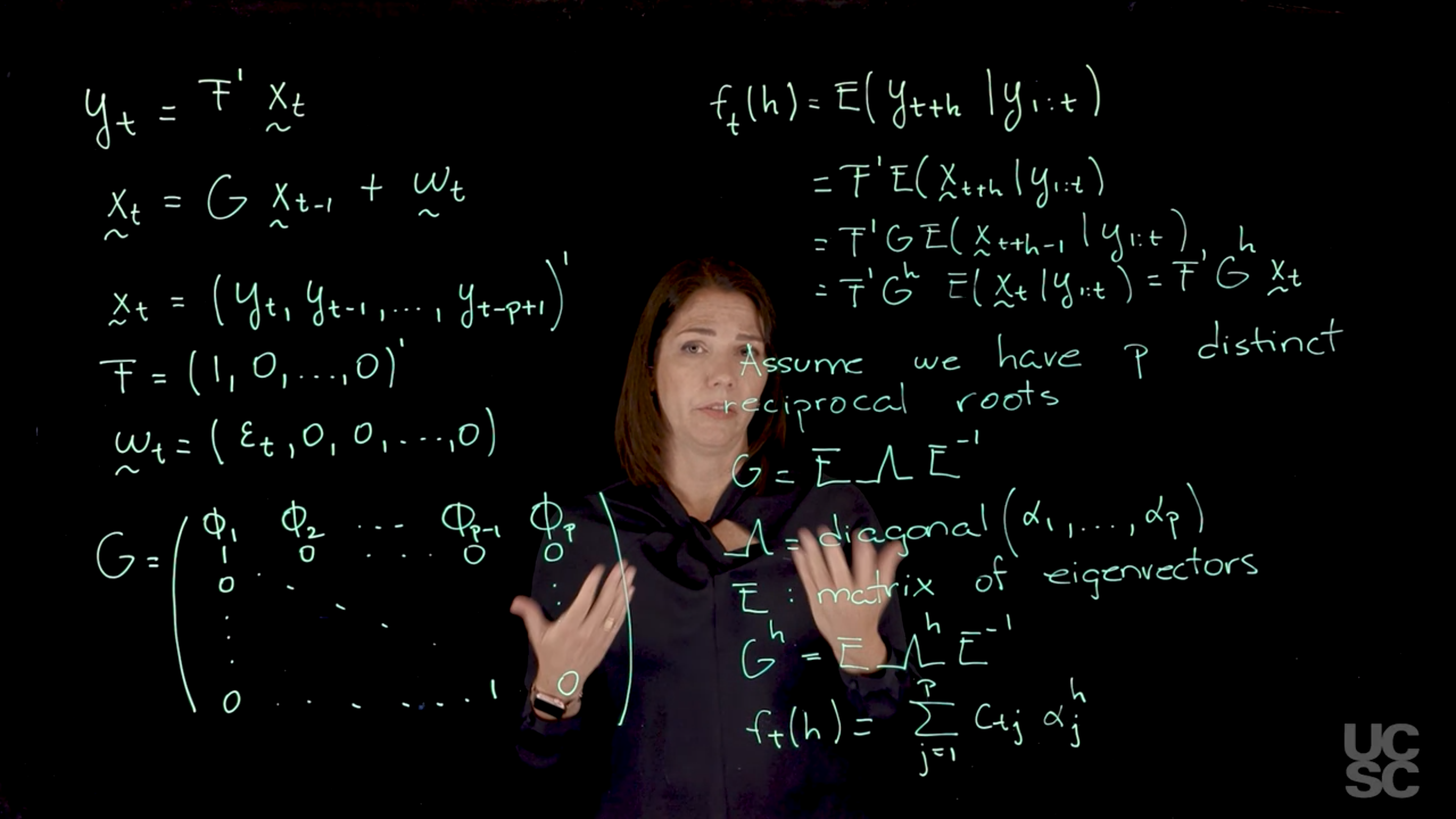
We will now discuss another important representation of the AR(P) process, one that is based on a state-space representation of the process. Again, we care about this type of representations because they allow us to study some important properties of the process. In this case, our state-space or dynamic linear model representation, we will make some connections with these representations later when we talk about dynamic linear models, is given as follows for an AR(P). I have my y_t. I can write it as F transpose and then another vector x_t here. Then we’re going to have x_t is going to be a function of x_t minus 1. That vector there is going to be an F and a G. I will describe what those are in a second. Then I’m going to have another vector here with some distribution. In our case, we are going to have a normal distribution also for that one. In the case of the AR(P), we’re going to have x_t to be y_t, y_t minus 1. >It’s a vector that has all these values of the y_t process. Then F is going to be a vector. It has to match the dimension of this vector. The first entry is going to be a one, and then I’m going to have zeros everywhere else. The w here is going to be a vector as well. > >The first component is going to be the Epsilon t. That we defined for the ARP process. Then every other entry is going to be a zero here. Again, the dimensions are going to match so that I get the right equations here. Then finally, my G matrix in this representation is going to be a very important matrix, the first row is going to contain the AR parameters, the AR coefficients. >We have p of those. That’s my first row. In this block, I’m going to have an identity matrix. It’s going to have ones in the diagonal and zeros everywhere else. I’m going to have a one here, and then I want to have zeros everywhere else. In this portion, I’m going to have column vector here of zeros. This is my G matrix. Why is this G matrix important? This G matrix is going to be related to the characteristic polynomial, in particular, is going to be related to the reciprocal roots of the characteristic polynomial that we discussed before. The eigenvalues of this matrix correspond precisely to the reciprocal roots of the characteristic polynomial. We will think about that and write down another representation related to this process. But before we go there, I just want you to look at this equation and see that if you do the matrix operations that are described these two equations, you get back the form of your autoregressive process. The other thing is, again, this is called a state-space representation because you have two equations here. One, you can call it the observational level equation where you are relating your observed y’s with some other model information here. Then there is another equation that has a Markovian structure here, where x_t is a function of x_t minus 1. This is why this is a state-space representation. One of the nice things about working with this representation is we can use some definitions that apply to dynamic linear models or state-space models, and one of those definitions is the so-called forecast function. The forecast function, we can define it in terms of, I’m going to use here the notation f_t h to denote that is a function f that depends on the time t that you’re considering, and then you’re looking at forecasting h steps ahead in your time series. If you have observations up to today and you want to look at what is the forecast function five days later, you will have h equals 5 there. It’s just the expected value. We are going to think of this as the expected value of y_t plus h. Conditional on all the observations or all the information you have received up to time t. I’m going to write it just like this. Using the state-space representation, you can see that if I use the first equation and I think about the expected value of y_t plus h is going to be F transpose, and then I have the expected value of the vector x_t plus h in that case. I can think of just applying this, then I would have expected value of x_t plus h given y_1 up to t. But now when I look at the structure of x_t plus h, if I go to my second equation here, I can see that x_t plus h is going to be dependent on x_t plus h minus 1, and there is a G matrix here. I can write this in terms of the expected value of x_t plus h, which is just G, expected value of x_t plus h minus 1, and then I also have plus expected value of the w_t’s. But because of the structure of the AR process that we defined, we said that all the Epsilon T’s are independent normally distributed random variables center at zero. In this case, those are going to be all zero. I can write down this as F transpose G, and then I have the expected value of x_t plus h minus 1 given y_1 up to t. If I continue with this process all the way until I get to time t, I’m going to get a product of all these G matrices here, and because we are starting with this lag h, I’m going to have the product of that G matrix h times. I can write this down as F transpose G to the power of h, and then I’m going to have the expected value of, finally, I get up to here. > >This is simply is going to be just my x_t vector. I can write this down as F transpose G^h, and then I have just my x_t. Again, why do we care? Now we are going to make that connection with this matrix and the eigenstructure of this matrix. I said before, one of the features of this matrix is that the eigenstructure is related to the reciprocal roots of the characteristic polynomial. In particular, the eigenvalues of this matrix correspond to the reciprocal roots of the characteristic polynomial. If we are working with the case in which we have exactly p different roots. We have as many different roots as the order of the AR process. Let’s say, p distinct. >We can write down then G in terms of its eigendecomposition. I can write this down as E, a matrix Lambda here, E inverse. > >Here, Lambda is going to be a diagonal matrix, >you just put the reciprocal roots, I’m going to call those Alpha 1 up to Alpha p. They are all different. You just put them in the diagonal and you can use any order you want. But the eigendecomposition, the eigenvectors, have to follow the order that you choose for the eigenvalues. Then what happens is, regardless of that, you’re going to have a unique G. But here, the E is a matrix of eigenvectors.

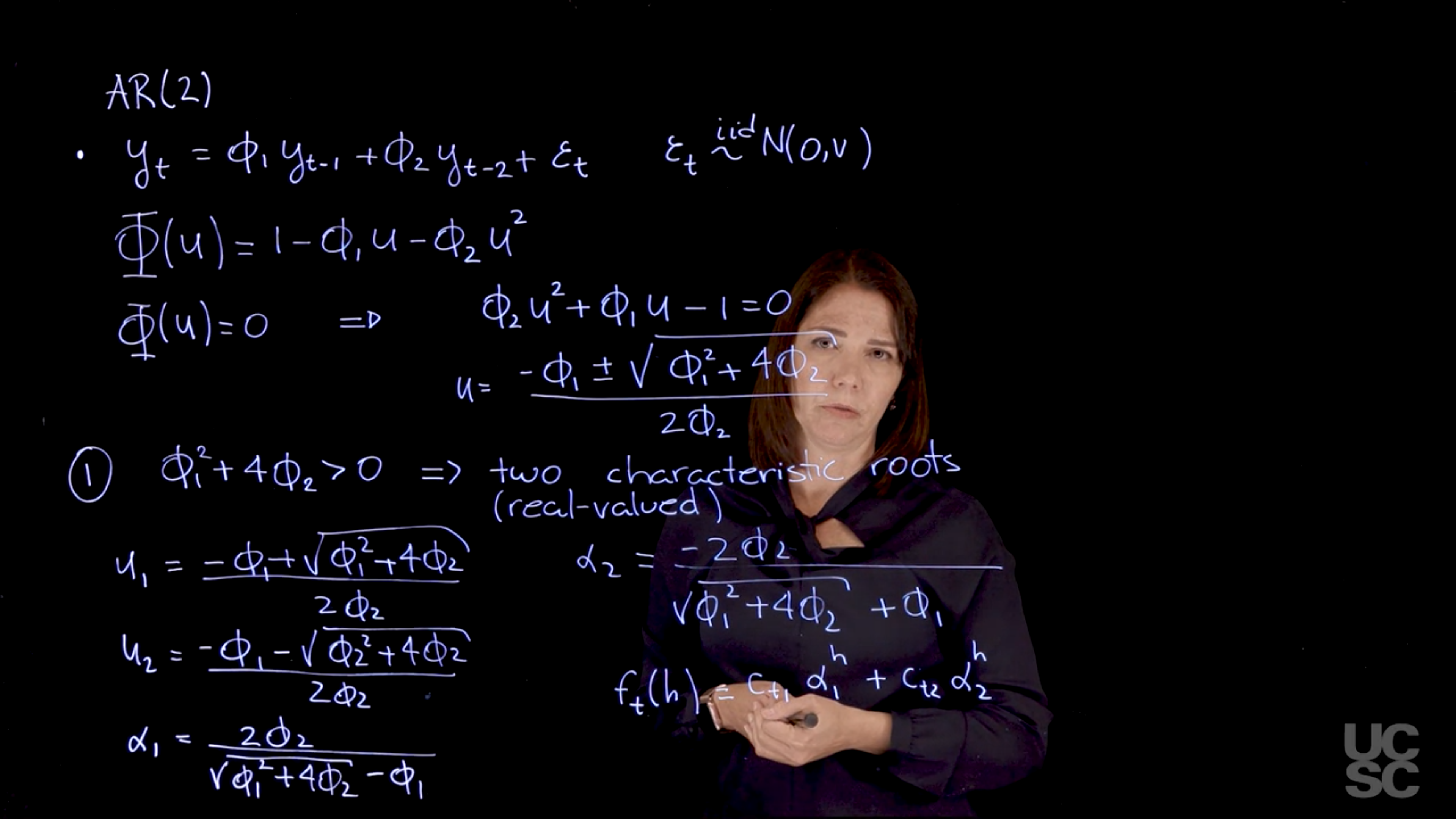
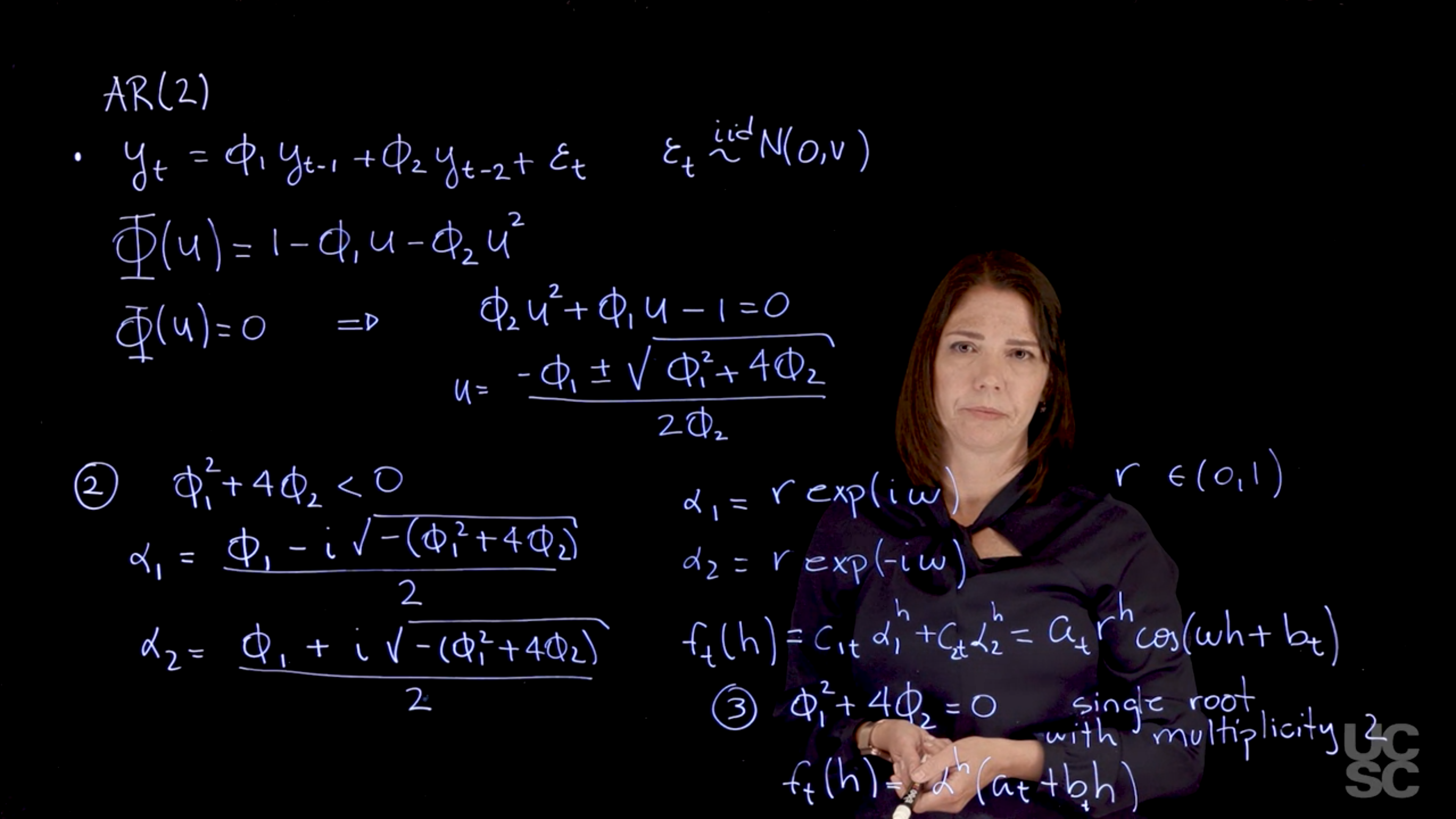
Again, why do we care? Well, if you look at what we have here, we have the power G to the power of h. Using that eigendecomposition, we can get to write this in this form. Whatever elements you have in the matrix of eigenvectors, they are now going to be functions of the reciprocal roots. The power that appears here, which is the number of steps ahead that you want to forecast in your time series for prediction, I’m just going to have the Alphas to the power of h. When I do this calculation, I can end up writing the forecast function just by doing that calculation as a sum from j equals 1 up to p of some constants. Those constants are going to be related to those E matrices but the important point is that what appears here is my Alpha to the power of h. What this means is I’m breaking this expected value of what I’m going to see in the future in terms of a function of the reciprocal roots of the characteristic polynomial. You can see that if the process is stable, is going to be stationary, all the moduli of my reciprocal roots are going to be below one. This is going to decay exponentially as a function of h. You’re going to have something that decays exponentially. Depending on whether those reciprocal roots are real-valued or complex-valued, you’re going to have behavior here that may be quasiperiodic for complex-valued roots or just non-quasiperiodic for the real valued roots. The other thing that matters is, if you’re working with a stable process, are going to have moduli smaller than one. The contribution of each of the roots to these forecasts function is going to be dependent on how close that modulus of that reciprocal root is to one or minus one. For roots that have relatively large values of the modulus, then they are going to have more contribution in terms of what’s going to happen in the future. This provides a way to interpret the AR process.

Examples (video)

AR(1)

AR(1)

AR(2) two positive roots

AR(2) two positive roots

AR(2) complex roots

AR(2) complex roots

Nulla eget cursus ipsum. Vivamus porttitor leo diam, sed volutpat lectus facilisis sit amet. Maecenas et pulvinar metus. Ut at dignissim tellus. In in tincidunt elit. Etiam vulputate lobortis arcu, vel faucibus leo lobortis ac. Aliquam erat volutpat. In interdum orci ac est euismod euismod. Nunc eleifend tristique risus, at lacinia odio commodo in. Sed aliquet ligula odio, sed tempor neque ultricies sit amet.

Etiam quis tortor luctus, pellentesque ante a, finibus dolor. Phasellus in nibh et magna pulvinar malesuada. Ut nisl ex, sagittis at sollicitudin et, sollicitudin id nunc. In id porta urna. Proin porta dolor dolor, vel dapibus nisi lacinia in. Pellentesque ante mauris, ornare non euismod a, fermentum ut sapien. Proin sed vehicula enim. Aliquam tortor odio, vestibulum vitae odio in, tempor molestie justo. Praesent maximus lacus nec leo maximus blandit.

Maecenas turpis velit, ultricies non elementum vel, luctus nec nunc. Nulla a diam interdum, faucibus sapien viverra, finibus metus. Donec non tortor diam. In ut elit aliquet, bibendum sem et, aliquam tortor. Donec congue, sem at rhoncus ultrices, nunc augue cursus erat, quis porttitor mauris libero ut ex. Nullam quis leo urna. Donec faucibus ligula eget pellentesque interdum. Lorem ipsum dolor sit amet, consectetur adipiscing elit. Aenean rhoncus interdum erat ut ultricies. Aenean tempus ex non elit suscipit, quis dignissim enim efficitur. Proin laoreet enim massa, vitae laoreet nulla mollis quis.

ACF of the AR(p) (video)

ACF of the AR(p)

ACF of the AR(p)

Nunc ac dignissim magna. Vestibulum vitae egestas elit. Proin feugiat leo quis ante condimentum, eu ornare mauris feugiat. Pellentesque habitant morbi tristique senectus et netus et malesuada fames ac turpis egestas. Mauris cursus laoreet ex, dignissim bibendum est posuere iaculis. Suspendisse et maximus elit. In fringilla gravida ornare. Aenean id lectus pulvinar, sagittis felis nec, rutrum risus. Nam vel neque eu arcu blandit fringilla et in quam. Aliquam luctus est sit amet vestibulum eleifend. Phasellus elementum sagittis molestie. Proin tempor lorem arcu, at condimentum purus volutpat eu. Fusce et pellentesque ligula. Pellentesque id tellus at erat luctus fringilla. Suspendisse potenti.

Etiam maximus accumsan gravida. Maecenas at nunc dignissim, euismod enim ac, bibendum ipsum. Maecenas vehicula velit in nisl aliquet ultricies. Nam eget massa interdum, maximus arcu vel, pretium erat. Maecenas sit amet tempor purus, vitae aliquet nunc. Vivamus cursus urna velit, eleifend dictum magna laoreet ut. Duis eu erat mollis, blandit magna id, tincidunt ipsum. Integer massa nibh, commodo eu ex vel, venenatis efficitur ligula. Integer convallis lacus elit, maximus eleifend lacus ornare ac. Vestibulum scelerisque viverra urna id lacinia. Vestibulum ante ipsum primis in faucibus orci luctus et ultrices posuere cubilia curae; Aenean eget enim at diam bibendum tincidunt eu non purus. Nullam id magna ultrices, sodales metus viverra, tempus turpis.

Simulating data from an AR(p) (video)

Proin sodales neque erat, varius cursus diam tincidunt sit amet. Etiam scelerisque fringilla nisl eu venenatis. Donec sem ipsum, scelerisque ac venenatis quis, hendrerit vel mauris. Praesent semper erat sit amet purus condimentum, sit amet auctor mi feugiat. In hac habitasse platea dictumst. Nunc ac mauris in massa feugiat bibendum id in dui. Praesent accumsan urna at lacinia aliquet. Proin ultricies eu est quis pellentesque. In vel lorem at nisl rhoncus cursus eu quis mi. In eu rutrum ante, quis placerat justo. Etiam euismod nibh nibh, sed elementum nunc imperdiet in. Praesent gravida nunc vel odio lacinia, at tempus nisl placerat. Aenean id ipsum sed est sagittis hendrerit non in tortor.

Lorem ipsum dolor sit amet, consectetur adipiscing elit. Duis sagittis posuere ligula sit amet lacinia. Duis dignissim pellentesque magna, rhoncus congue sapien finibus mollis. Ut eu sem laoreet, vehicula ipsum in, convallis erat. Vestibulum magna sem, blandit pulvinar augue sit amet, auctor malesuada sapien. Nullam faucibus leo eget eros hendrerit, non laoreet ipsum lacinia. Curabitur cursus diam elit, non tempus ante volutpat a. Quisque hendrerit blandit purus non fringilla. Integer sit amet elit viverra ante dapibus semper. Vestibulum viverra rutrum enim, at luctus enim posuere eu. Orci varius natoque penatibus et magnis dis parturient montes, nascetur ridiculus mus.

Computing the roots of the AR polynomial (reading)

Compute AR reciprocal roots given the AR coefficients

Code
# Assume the folloing AR coefficients for an AR(8)
phi=c(0.27, 0.07, -0.13, -0.15, -0.11, -0.15, -0.23, -0.14)
roots=1/polyroot(c(1, -phi)) # compute reciprocal characteristic roots
r=Mod(roots) # compute moduli of reciprocal roots
lambda=2*pi/Arg(roots) # compute periods of reciprocal roots

# print results modulus and frequency by decreasing order
print(cbind(r, abs(lambda))[order(r, decreasing=TRUE), ][c(2,4,6,8),]) 
             r          
[1,] 0.9722428 12.731401
[2,] 0.8094950  5.103178
[3,] 0.7196221  2.987712
[4,] 0.6606487  2.232193

Simulating data from an AR(p) (reading)

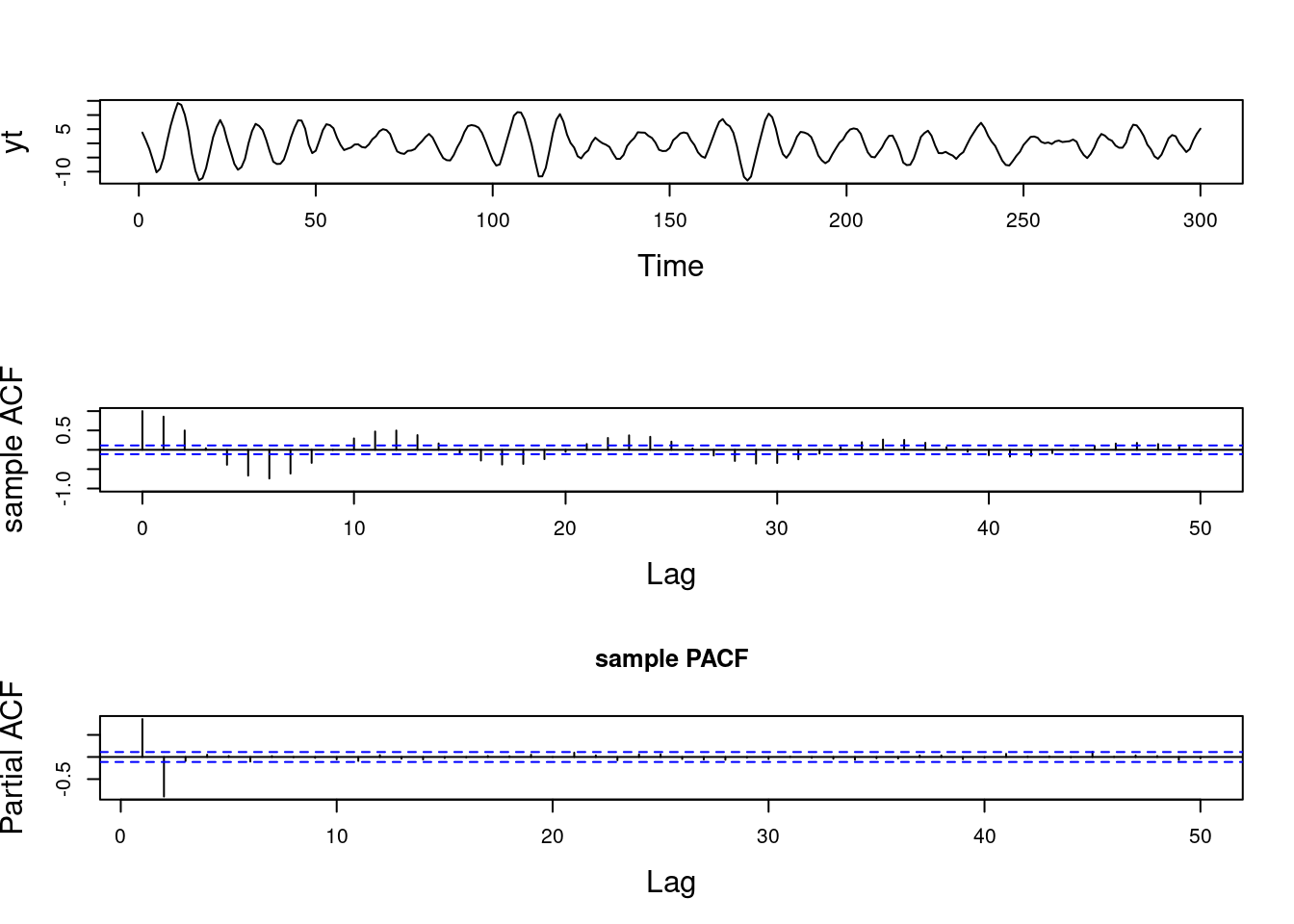
  1. Rcode to simulate data from an AR(2) with one pair of complex-valued reciprocal roots and plot the corresponding sample ACF and sample PACF
Code
## simulate data from an AR(2)
set.seed(2021)
## AR(2) with a pair of complex-valued roots with modulus 0.95 and period 12 
r=0.95
lambda=12 
phi=numeric(2) 
phi[1]<- 2*r*cos(2*pi/lambda) 
phi[2] <- -r^2
phi
[1]  1.645448 -0.902500
Code
T=300 # number of time points
sd=1 # innovation standard deviation
yt=arima.sim(n=T, model = list(ar = phi), sd=sd)

par(mfrow = c(3, 1), cex.lab = 1.5)
## plot simulated data 
ts.plot(yt)
## draw sample autocorrelation function
acf(yt, lag.max = 50,
    type = "correlation", ylab = "sample ACF", 
    lty = 1, ylim = c(-1, 1), main = " ")

## draw sample partial autocorrelation function
pacf(yt, lag.ma = 50, main = "sample PACF")

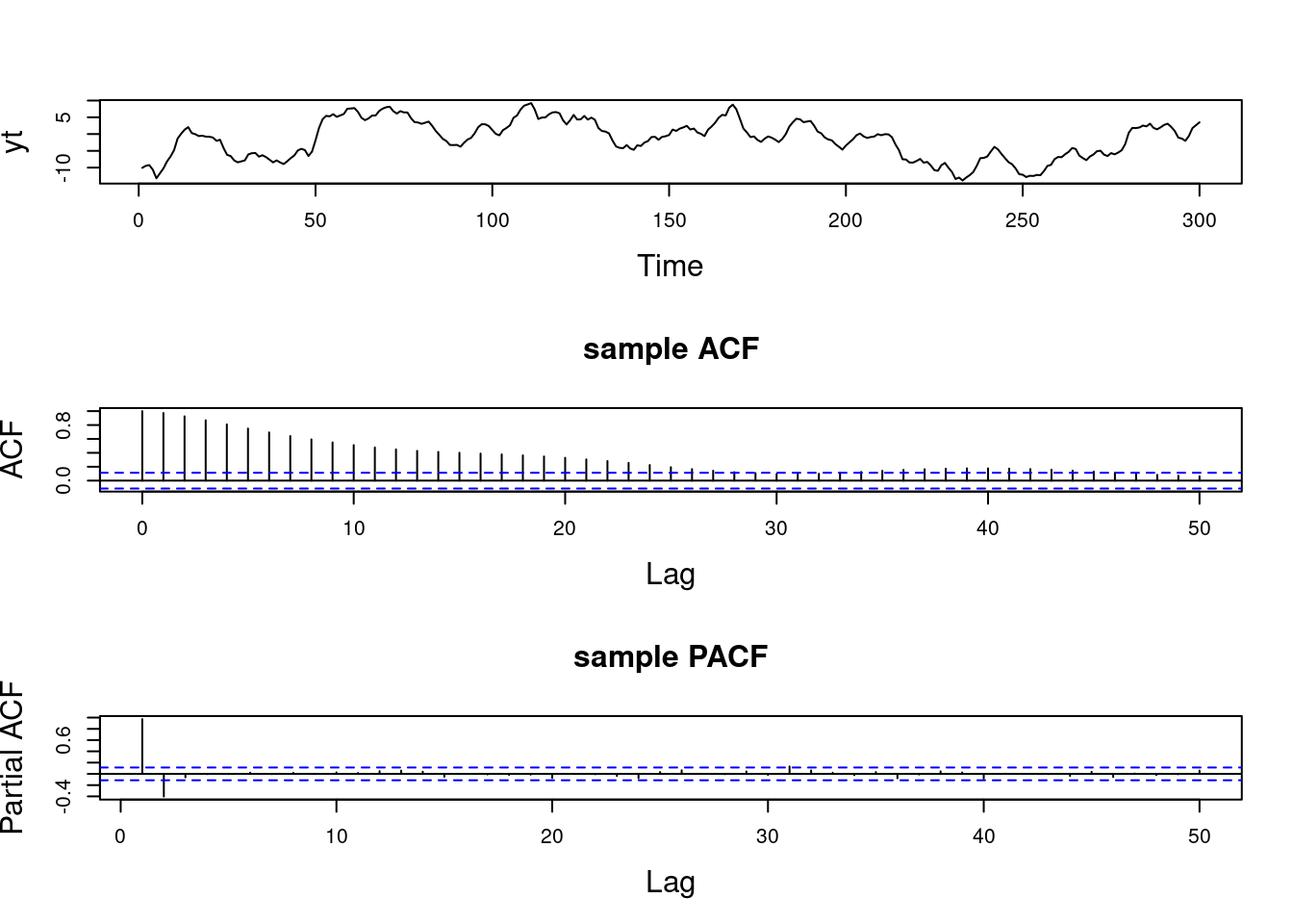
  1. Rcode to simulate data from an AR(2) with two different real-valued reciprocal roots and plot the corresponding sample ACF and sample PACF
Code
### Simulate from AR(2) with two real reciprocal roots (e.g., 0.95 and 0.5)
set.seed(2021)
recip_roots=c(0.95, 0.5) ## two different real reciprocal roots
phi=c(sum(recip_roots), -prod(recip_roots)) ## compute ar coefficients
phi
[1]  1.450 -0.475
Code
T=300 ## set up number of time points
sd=1 ## set up standard deviation
yt=arima.sim(n=T,model = list(ar=phi),sd=sd) # generate ar(2)

par(mfrow = c(3, 1), cex.lab = 1.5, cex.main = 1.5)
### plot simulated data 
ts.plot(yt)
### plot sample ACF
acf(yt, lag.max = 50, type = "correlation",  main = "sample ACF")
### plot sample PACF
pacf(yt, lag.max = 50, main = "sample PACF")

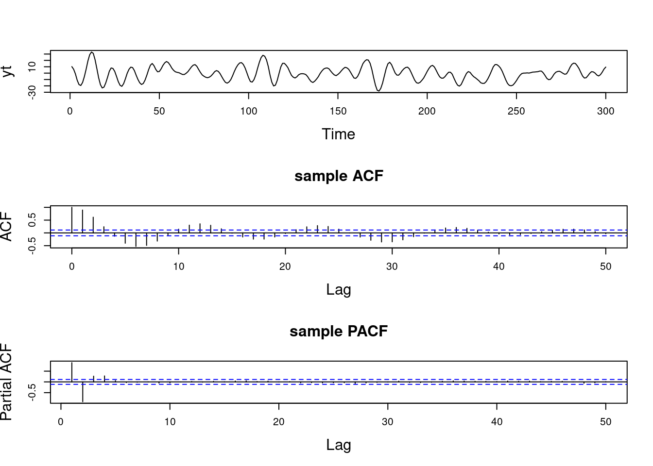
  1. Rcode to simulate data from an AR(3) with one real reciprocal root and a pair of complex-valued reciprocal roots and plot the corresponding sample ACF and sample PACF
Code
### Simulate from AR(3) with one real root 
### and a pair of complex roots (e.g., r=0.95 and lambda = 12 and real root with
### 0.8 modulus)
set.seed(2021)
r= c(0.95, 0.95, 0.8) ## modulus
lambda=c(-12, 12) ## lambda
recip_roots=c(r[1:2]*exp(2*pi/lambda*1i), r[3]) ## reciprocal roots
phi <- numeric(3) # placeholder for phi
phi[1]=Re(sum(recip_roots)) # ar coefficients at lag 1
phi[2]=-Re(recip_roots[1]*recip_roots[2] + recip_roots[1]*recip_roots[3] + recip_roots[2]*recip_roots[3]) # ar coefficients at lag 2
phi[3]=Re(prod(recip_roots))
phi
[1]  2.445448 -2.218859  0.722000
Code
T=300 # number of time points
sd=1 # standard deviation
yt=arima.sim(n=T,model = list(ar=phi), sd = sd) # generate ar(3)

par(mfrow = c(3,1), cex.lab = 1.5, cex.main = 1.5)
### plot simulated data 
ts.plot(yt)
### plot sample ACF
acf(yt, lag.max = 50, type = "correlation",  main = "sample ACF")
### plot sample PACF
pacf(yt, lag.max = 50, main = "sample PACF")

The AR(p): Review (Reading)

AR(p): Definition, stability, and stationarity

AR(p)

A time series follows a zero-mean autoregressive process of order p, of AR(p), if:

y_t = \phi_1 y_{t-1} + \phi_2 y_{t-2} + \ldots + \phi_p y_{t-p} + \epsilon_t \qquad \tag{5}

where \phi_1, \ldots, \phi_p are the AR coefficients and \epsilon_t is a white noise process

with \epsilon_t \sim \text{i.i.d. } N(0, v), for all t.

The AR characteristic polynomial is given by

\Phi(u) = 1 - \phi_1 u - \phi_2 u^2 - \ldots - \phi_p u^p,

with u complex-valued.

The AR(p) process is stable if \Phi(u) = 0 only when |u| > 1. In this case, the process is also stationary and can be written as

y_t = \psi(B) \epsilon_t = \sum_{j=0}^{\infty} \psi_j \epsilon_{t-j},

with \psi_0 = 1 and \sum_{j=0}^{\infty} |\psi_j| < \infty. Here B denotes the backshift operator, so B^j \epsilon_t = \epsilon_{t-j} and

\psi(B) = 1 + \psi_1 B + \psi_2 B^2 + \ldots + \psi_j B^j + \ldots

The AR polynomial can also be written as

\Phi(u) = \prod_{j=1}^{p} (1 - \alpha_j u),

with \alpha_j being the reciprocal roots of the characteristic polynomial. For the process to be stable (and consequently stationary), |\alpha_j| < 1 for all j = 1, \ldots, p.

AR(p): State-space representation

An AR(p) can also be represented using the following state-space or dynamic linear (DLM) model representation:

y_t = F' x_t,

x_t = G x_{t-1} + \omega_t,

with x_t = (y_t, y_{t-1}, \dots, y_{t-p+1})', F = (1, 0, \dots, 0)', \omega_t = (\epsilon_t, 0, \dots, 0)', and

G = \begin{pmatrix} \phi_1 & \phi_2 & \phi_3 & \dots & \phi_{p-1} & \phi_p \\ 1 & 0 & 0 & \dots & 0 & 0 \\ 0 & 1 & 0 & \dots & 0 & 0 \\ \vdots & \ddots & \ddots & \ddots & & \vdots \\ 0 & 0 & 0 & \dots & 1 & 0 \end{pmatrix}.

Using this representation, the expected behavior of the process in the future can be exhibited via the forecast function:

f_t(h) = E(y_{t+h} | y_{1:t}) = F' G^h x_t, \quad h > 0,

for any t \ge p. The eigenvalues of the matrix G are the reciprocal roots of the characteristic polynomial.

Eigenvalues
  • The eigenvalues can be real-valued or complex-valued.
  • If they are Complex-valued the eigenvalues/reciprocal roots appear in conjugate pairs.

Assuming the matrix G has p distinct eigenvalues, we can decompose G into G = E \Lambda E^{-1}, with

\Lambda = \text{diag}(\alpha_1, \dots, \alpha_p),

for a matrix of corresponding eigenvectors E. Then, G^h = E \Lambda^h E^{-1} and we have:

f_t(h) = \sum_{j=1}^{p} c_{tj} \alpha_j^h.

ACF of AR(p)

For a general AR(p), the ACF is given in terms of the homogeneous difference equation:

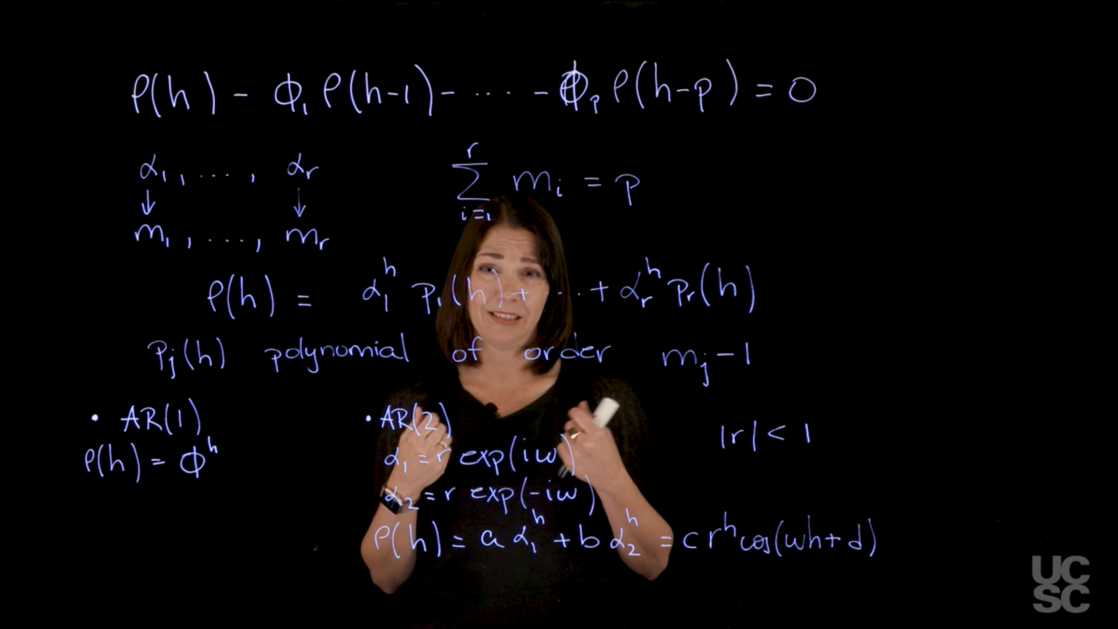
\rho(h) - \phi_1 \rho(h-1) - \ldots - \phi_p \rho(h-p) = 0, \quad h > 0.

Assuming that \alpha_1, \dots, \alpha_r denotes the characteristic reciprocal roots each with multiplicity m_1, \ldots, m_r, respectively, with \sum_{i=1}^{r} m_i = p. Then, the general solution is

\rho(h) = \alpha_1^h p_1(h) + \ldots + \alpha_r^h p_r(h),

with p_j(h) being a polynomial of degree m_j - 1.

Example: AR(1)

We already know that for h \ge 0, \rho(h) = \phi^h. Using the result above, we have

\rho(h) = a \phi^h,

and so to find a, we take \rho(0) = 1 = a \phi^0, hence a = 1.

Example: AR(2)

Similarly, using the result above in the case of two complex-valued reciprocal roots, we have

\rho(h) = a \alpha_1^h + b \alpha_2^h = c r^h \cos(\omega h + d).

PACF of AR(p)

We can use the Durbin-Levinson recursion to obtain the PACF of an AR(p).

Using the same representation but substituting the true autocovariances and autocorrelations with their sampled versions, we can also obtain the sample PACF.

It is possible to show that the PACF of an AR(p) is equal to zero for h > p.

Quiz: The AR(p) process (Quiz)

Omitted due to Coursera’s Honor Code
Bayesian Inference in the AR(p)

Bayesian inference in the AR(p): Reference prior, conditional likelihood (video)

Ut ut condimentum augue, nec eleifend nisl. Sed facilisis egestas odio ac pretium. Pellentesque consequat magna sed venenatis sagittis. Vivamus feugiat lobortis magna vitae accumsan. Pellentesque euismod malesuada hendrerit. Ut non mauris non arcu condimentum sodales vitae vitae dolor. Nullam dapibus, velit eget lacinia rutrum, ipsum justo malesuada odio, et lobortis sapien magna vel lacus. Nulla purus neque, hendrerit non malesuada eget, mattis vel erat. Suspendisse potenti.

Nullam dapibus cursus dolor sit amet consequat. Nulla facilisi. Curabitur vel nulla non magna lacinia tincidunt. Duis porttitor quam leo, et blandit velit efficitur ut. Etiam auctor tincidunt porttitor. Phasellus sed accumsan mi. Fusce ut erat dui. Suspendisse eu augue eget turpis condimentum finibus eu non lorem. Donec finibus eros eu ante condimentum, sed pharetra sapien sagittis. Phasellus non dolor ac ante mollis auctor nec et sapien. Pellentesque vulputate at nisi eu tincidunt. Vestibulum at dolor aliquam, hendrerit purus eu, eleifend massa. Morbi consectetur eros id tincidunt gravida. Fusce ut enim quis orci hendrerit lacinia sed vitae enim.

Rcode: Maximum likelihood estimation, AR(p), conditional likelihood (Reading)

Code
  set.seed(2021)
# Simulate 300 observations from an AR(2) with one pair of complex-valued reciprocal roots 
r=0.95
lambda=12 
phi=numeric(2) 
phi[1]=2*r*cos(2*pi/lambda) 
phi[2]=-r^2
sd=1 # innovation standard deviation
T=300 # number of time points
# generate stationary AR(2) process
yt=arima.sim(n = T, model = list(ar = phi), sd = sd) 

## Compute the MLE for phi and the unbiased estimator for v using the conditional likelihood
p=2
y=rev(yt[(p+1):T]) # response
X=t(matrix(yt[rev(rep((1:p),T-p)+rep((0:(T-p-1)),rep(p,T-p)))],p,T-p));
XtX=t(X)%*%X
XtX_inv=solve(XtX)
phi_MLE=XtX_inv%*%t(X)%*%y # MLE for phi
s2=sum((y - X%*%phi_MLE)^2)/(length(y) - p) #unbiased estimate for v

cat("\n MLE of conditional likelihood for phi: ", phi_MLE, "\n",
    "Estimate for v: ", s2, "\n")

 MLE of conditional likelihood for phi:  1.65272 -0.9189823 
 Estimate for v:  0.9901292 

Model order selection (video)

Lorem ipsum dolor sit amet, consectetur adipiscing elit. Duis sagittis posuere ligula sit amet lacinia. Duis dignissim pellentesque magna, rhoncus congue sapien finibus mollis. Ut eu sem laoreet, vehicula ipsum in, convallis erat. Vestibulum magna sem, blandit pulvinar augue sit amet, auctor malesuada sapien. Nullam faucibus leo eget eros hendrerit, non laoreet ipsum lacinia. Curabitur cursus diam elit, non tempus ante volutpat a. Quisque hendrerit blandit purus non fringilla. Integer sit amet elit viverra ante dapibus semper. Vestibulum viverra rutrum enim, at luctus enim posuere eu. Orci varius natoque penatibus et magnis dis parturient montes, nascetur ridiculus mus.

Nunc ac dignissim magna. Vestibulum vitae egestas elit. Proin feugiat leo quis ante condimentum, eu ornare mauris feugiat. Pellentesque habitant morbi tristique senectus et netus et malesuada fames ac turpis egestas. Mauris cursus laoreet ex, dignissim bibendum est posuere iaculis. Suspendisse et maximus elit. In fringilla gravida ornare. Aenean id lectus pulvinar, sagittis felis nec, rutrum risus. Nam vel neque eu arcu blandit fringilla et in quam. Aliquam luctus est sit amet vestibulum eleifend. Phasellus elementum sagittis molestie. Proin tempor lorem arcu, at condimentum purus volutpat eu. Fusce et pellentesque ligula. Pellentesque id tellus at erat luctus fringilla. Suspendisse potenti.

Example: Bayesian inference in the AR(p), conditional likelihood (Video)

Etiam quis tortor luctus, pellentesque ante a, finibus dolor. Phasellus in nibh et magna pulvinar malesuada. Ut nisl ex, sagittis at sollicitudin et, sollicitudin id nunc. In id porta urna. Proin porta dolor dolor, vel dapibus nisi lacinia in. Pellentesque ante mauris, ornare non euismod a, fermentum ut sapien. Proin sed vehicula enim. Aliquam tortor odio, vestibulum vitae odio in, tempor molestie justo. Praesent maximus lacus nec leo maximus blandit.

Maecenas turpis velit, ultricies non elementum vel, luctus nec nunc. Nulla a diam interdum, faucibus sapien viverra, finibus metus. Donec non tortor diam. In ut elit aliquet, bibendum sem et, aliquam tortor. Donec congue, sem at rhoncus ultrices, nunc augue cursus erat, quis porttitor mauris libero ut ex. Nullam quis leo urna. Donec faucibus ligula eget pellentesque interdum. Lorem ipsum dolor sit amet, consectetur adipiscing elit. Aenean rhoncus interdum erat ut ultricies. Aenean tempus ex non elit suscipit, quis dignissim enim efficitur. Proin laoreet enim massa, vitae laoreet nulla mollis quis.

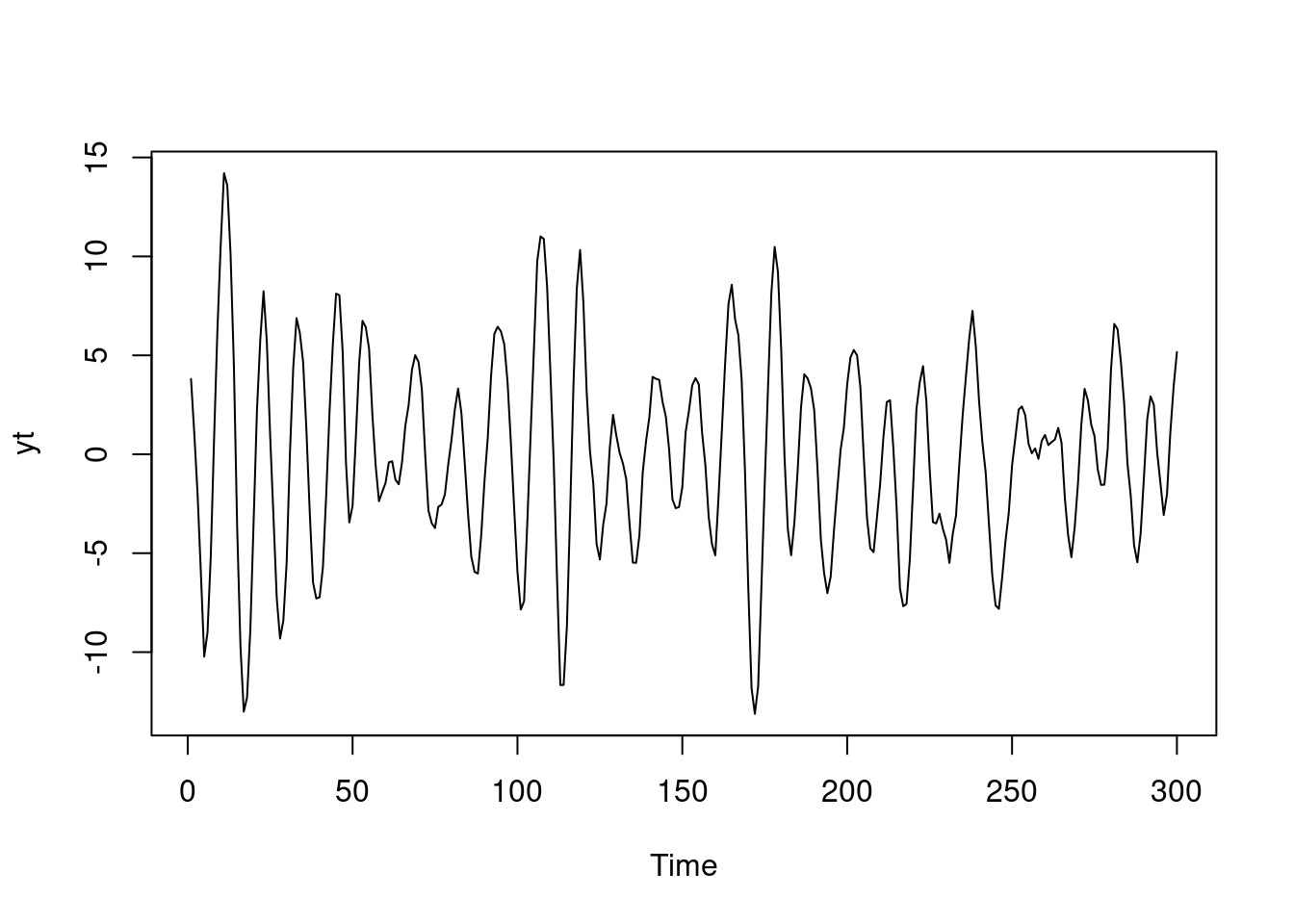
Rcode: Bayesian inference, AR(p), conditional likelihood (Reading)

Code
# Simulate 300 observations from an AR(2) with one pair of complex-valued roots 
set.seed(2021)
r=0.95
lambda=12 
phi=numeric(2) 
phi[1]=2*r*cos(2*pi/lambda) 
phi[2]=-r^2
sd=1 # innovation standard deviation
T=300 # number of time points
# generate stationary AR(2) process
yt=arima.sim(n = T, model = list(ar = phi), sd = sd) 
par(mfrow=c(1,1))
plot(yt)

Code
## Compute the MLE of phi and the unbiased estimator of v using the conditional likelihood
p=2
y=rev(yt[(p+1):T]) # response
X=t(matrix(yt[rev(rep((1:p),T-p)+rep((0:(T-p-1)),rep(p,T-p)))],p,T-p));
XtX=t(X)%*%X
XtX_inv=solve(XtX)
phi_MLE=XtX_inv%*%t(X)%*%y # MLE for phi
s2=sum((y - X%*%phi_MLE)^2)/(length(y) - p) #unbiased estimate for v

#####################################################################################
### Posterior inference, conditional likelihood + reference prior via 
### direct sampling                 
#####################################################################################

n_sample=1000 # posterior sample size
library(MASS)

## step 1: sample v from inverse gamma distribution
v_sample=1/rgamma(n_sample, (T-2*p)/2, sum((y-X%*%phi_MLE)^2)/2)

## step 2: sample phi conditional on v from normal distribution
phi_sample=matrix(0, nrow = n_sample, ncol = p)
for(i in 1:n_sample){
  phi_sample[i, ]=mvrnorm(1,phi_MLE,Sigma=v_sample[i]*XtX_inv)
}

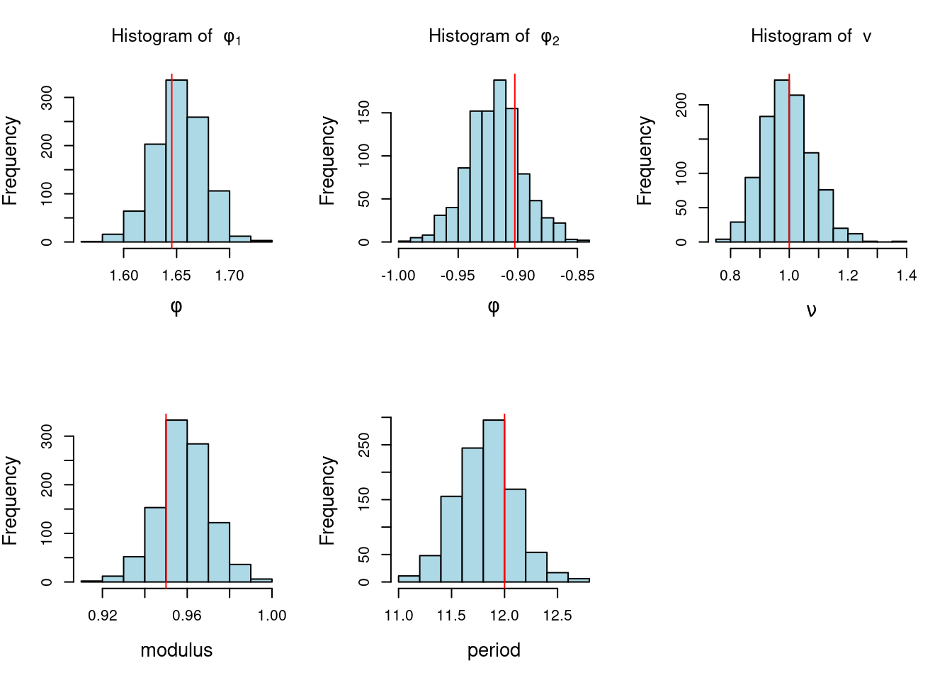
par(mfrow = c(2, 3), cex.lab = 1.3)
## plot histogram of posterior samples of phi and v

for(i in 1:2){
  hist(phi_sample[, i], xlab = bquote(phi), 
       main = bquote("Histogram of "~phi[.(i)]),col='lightblue')
  abline(v = phi[i], col = 'red')
}

hist(v_sample, xlab = bquote(nu), main = bquote("Histogram of "~v),col='lightblue')
abline(v = sd, col = 'red')

#####################################################
# Graph posterior for modulus and period 
#####################################################
r_sample=sqrt(-phi_sample[,2])
lambda_sample=2*pi/acos(phi_sample[,1]/(2*r_sample))
hist(r_sample,xlab="modulus",main="",col='lightblue')
abline(v=0.95,col='red')
hist(lambda_sample,xlab="period",main="",col='lightblue')
abline(v=12,col='red')

Rcode: Model order selection (Reading)

Code
###################################################
# Simulate data from an AR(2)
###################################################
set.seed(2021)
r=0.95
lambda=12 
phi=numeric(2) 
phi[1]=2*r*cos(2*pi/lambda) 
phi[2]=-r^2
sd=1 # innovation standard deviation
T=300 # number of time points
# generate stationary AR(2) process
yt=arima.sim(n = T, model = list(ar = phi), sd = sd) 

#############################################################################
######   compute AIC and BIC for different AR(p)s based on simulated data ###
#############################################################################
pmax=10 # the maximum of model order
Xall=t(matrix(yt[rev(rep((1:pmax),T-pmax)+rep((0:(T-pmax-1)),
              rep(pmax,T-pmax)))], pmax, T-pmax));
y=rev(yt[(pmax+1):T])
n_cond=length(y) # (number of total time points - the maximum of model order)

## compute MLE
my_MLE <- function(y, Xall, p){
  n=length(y)
  x=Xall[,1:p]
  a=solve(t(x) %*%x)
  a=(a + t(a))/2 # for numerical stability 
  b=a%*%t(x)%*%y # mle for ar coefficients
  r=y - x%*%b # residuals 
  nu=n - p # degrees freedom
  R=sum(r*r) # SSE
  s=R/nu #MSE
  return(list(b = b, s = s, R = R, nu = nu))
}


## function for AIC and BIC computation 
AIC_BIC <- function(y, Xall, p){
  ## number of time points
  n <- length(y)
  
  ## compute MLE
  tmp=my_MLE(y, Xall, p)
  
  ## retrieve results
  R=tmp$R
  
  ## compute likelihood
  likl= n*log(R)
  
  ## compute AIC and BIC
  aic =likl + 2*(p)
  bic =likl + log(n)*(p)
  return(list(aic = aic, bic = bic))
}
# Compute AIC, BIC 
aic =numeric(pmax)
bic =numeric(pmax)

for(p in 1:pmax){
  tmp =AIC_BIC(y,Xall, p)
  aic[p] =tmp$aic
  bic[p] =tmp$bic
  print(c(p, aic[p], bic[p])) # print AIC and BIC by model order
}
[1]    1.000 2166.793 2170.463
[1]    2.000 1635.816 1643.156
[1]    3.000 1637.527 1648.536
[1]    4.000 1639.059 1653.738
[1]    5.000 1640.743 1659.093
[1]    6.000 1641.472 1663.491
[1]    7.000 1643.457 1669.147
[1]    8.000 1645.370 1674.729
[1]    9.000 1646.261 1679.290
[1]   10.000 1647.915 1684.614
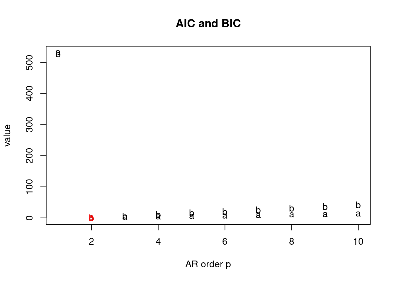
Code
## compute difference between the value and its minimum
aic =aic-min(aic) 
bic =bic-min(bic) 

## draw plot of AIC, BIC, and the marginal likelihood
par(mfrow = c(1, 1))
matplot(1:pmax,matrix(c(aic,bic),pmax,2),ylab='value',
        xlab='AR order p',pch="ab", col = 'black', main = "AIC and BIC")
# highlight the model order selected by AIC
text(which.min(aic), aic[which.min(aic)], "a", col = 'red') 
# highlight the model order selected by BIC
text(which.min(bic), bic[which.min(bic)], "b", col = 'red') 

Code
########################################################
p <- which.min(bic) # We set up the moder order
print(paste0("The chosen model order by BIC: ", p))
[1] "The chosen model order by BIC: 2"

Spectral representation of the AR(p) (video)

Praesent ornare dolor turpis, sed tincidunt nisl pretium eget. Curabitur sed iaculis ex, vitae tristique sapien. Quisque nec ex dolor. Quisque ut nisl a libero egestas molestie. Nulla vel porta nulla. Phasellus id pretium arcu. Etiam sed mi pellentesque nibh scelerisque elementum sed at urna. Ut congue molestie nibh, sit amet pretium ligula consectetur eu. Integer consectetur augue justo, at placerat erat posuere at. Ut elementum urna lectus, vitae bibendum neque pulvinar quis. Suspendisse vulputate cursus eros id maximus. Duis pulvinar facilisis massa, et condimentum est viverra congue. Curabitur ornare convallis nisl. Morbi dictum scelerisque turpis quis pellentesque. Etiam lectus risus, luctus lobortis risus ut, rutrum vulputate justo. Nulla facilisi.

Proin sodales neque erat, varius cursus diam tincidunt sit amet. Etiam scelerisque fringilla nisl eu venenatis. Donec sem ipsum, scelerisque ac venenatis quis, hendrerit vel mauris. Praesent semper erat sit amet purus condimentum, sit amet auctor mi feugiat. In hac habitasse platea dictumst. Nunc ac mauris in massa feugiat bibendum id in dui. Praesent accumsan urna at lacinia aliquet. Proin ultricies eu est quis pellentesque. In vel lorem at nisl rhoncus cursus eu quis mi. In eu rutrum ante, quis placerat justo. Etiam euismod nibh nibh, sed elementum nunc imperdiet in. Praesent gravida nunc vel odio lacinia, at tempus nisl placerat. Aenean id ipsum sed est sagittis hendrerit non in tortor.

Spectral representation of the AR(p): Example (video)

Vestibulum ultrices, tortor at mattis porta, odio nisi rutrum nulla, sit amet tincidunt eros quam facilisis tellus. Fusce eleifend lectus in elementum lacinia. Nam auctor nunc in massa ullamcorper, sit amet auctor ante accumsan. Nam ut varius metus. Curabitur eget tristique leo. Cras finibus euismod erat eget elementum. Integer vel placerat ex. Ut id eros quis lectus lacinia venenatis hendrerit vel ante.

Etiam congue quam eget velit convallis, eu sagittis orci vestibulum. Vestibulum at massa turpis. Curabitur ornare ex sed purus vulputate, vitae porta augue rhoncus. Phasellus auctor suscipit purus, vel ultricies nunc. Nunc eleifend nulla ac purus volutpat, id fringilla felis aliquet. Duis vitae porttitor nibh, in rhoncus risus. Vestibulum a est vitae est tristique vehicula. Proin mollis justo id est tempus hendrerit. Praesent suscipit placerat congue. Aliquam eu elit gravida, consequat augue non, ultricies sapien. Nunc ultricies viverra ante, sit amet vehicula ante volutpat id. Etiam tempus purus vitae tellus mollis viverra. Donec at ornare mauris. Aliquam sodales hendrerit ornare. Suspendisse accumsan lacinia sapien, sit amet imperdiet dui molestie ut.

Rcode: Spectral density of AR(p) (Reading)

Code
### Simulate 300 observations from an AR(2) prcess with a pair of complex-valued roots 
set.seed(2021)
r=0.95
lambda=12 
phi=numeric(2) 
phi[1]<- 2*r*cos(2*pi/lambda) 
phi[2] <- -r^2
sd=1 # innovation standard deviation
T=300 # number of time points
# sample from the AR(2) process
yt=arima.sim(n = T, model = list(ar = phi), sd = sd) 

# Compute the MLE of phi and the unbiased estimator of v using the conditional likelihood 
p=2
y=rev(yt[(p+1):T])
X=t(matrix(yt[rev(rep((1:p),T-p)+rep((0:(T-p-1)),rep(p,T-p)))],p,T-p));
XtX=t(X)%*%X
XtX_inv=solve(XtX)
phi_MLE=XtX_inv%*%t(X)%*%y # MLE for phi
s2=sum((y - X%*%phi_MLE)^2)/(length(y) - p) #unbiased estimate for v

# Obtain 200 samples from the posterior distribution under the conditional likelihood and the reference prior 
n_sample=200 # posterior sample size
library(MASS)

## step 1: sample v from inverse gamma distribution
v_sample=1/rgamma(n_sample, (T-2*p)/2, sum((y-X%*%phi_MLE)^2)/2)

## step 2: sample phi conditional on v from normal distribution
phi_sample=matrix(0, nrow = n_sample, ncol = p)
for(i in 1:n_sample){
  phi_sample[i,]=mvrnorm(1,phi_MLE,Sigma=v_sample[i]*XtX_inv)
}


### using spec.ar to draw spectral density based on the data assuming an AR(2)
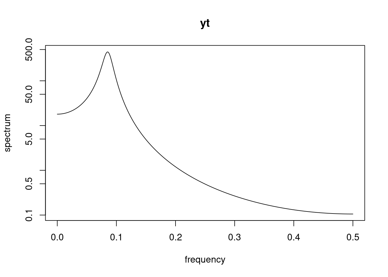
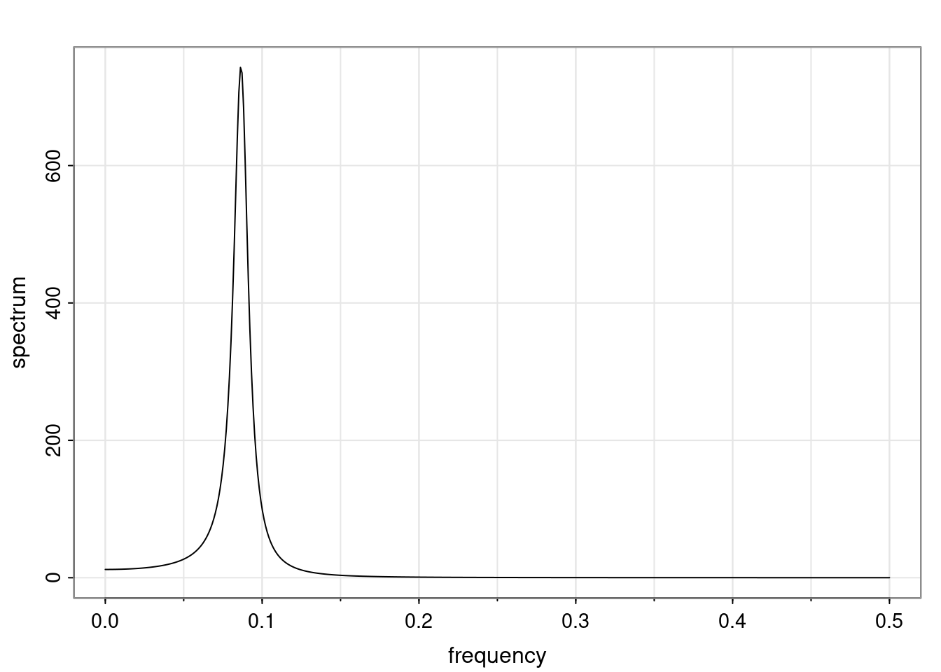
spec.ar(yt, order = 2, main = "yt")

Code
### using arma.spec from astsa package to draw spectral density
library("astsa")

## plot spectral density of simulated data with posterior sampled 
## ar coefficients and innvovation variance
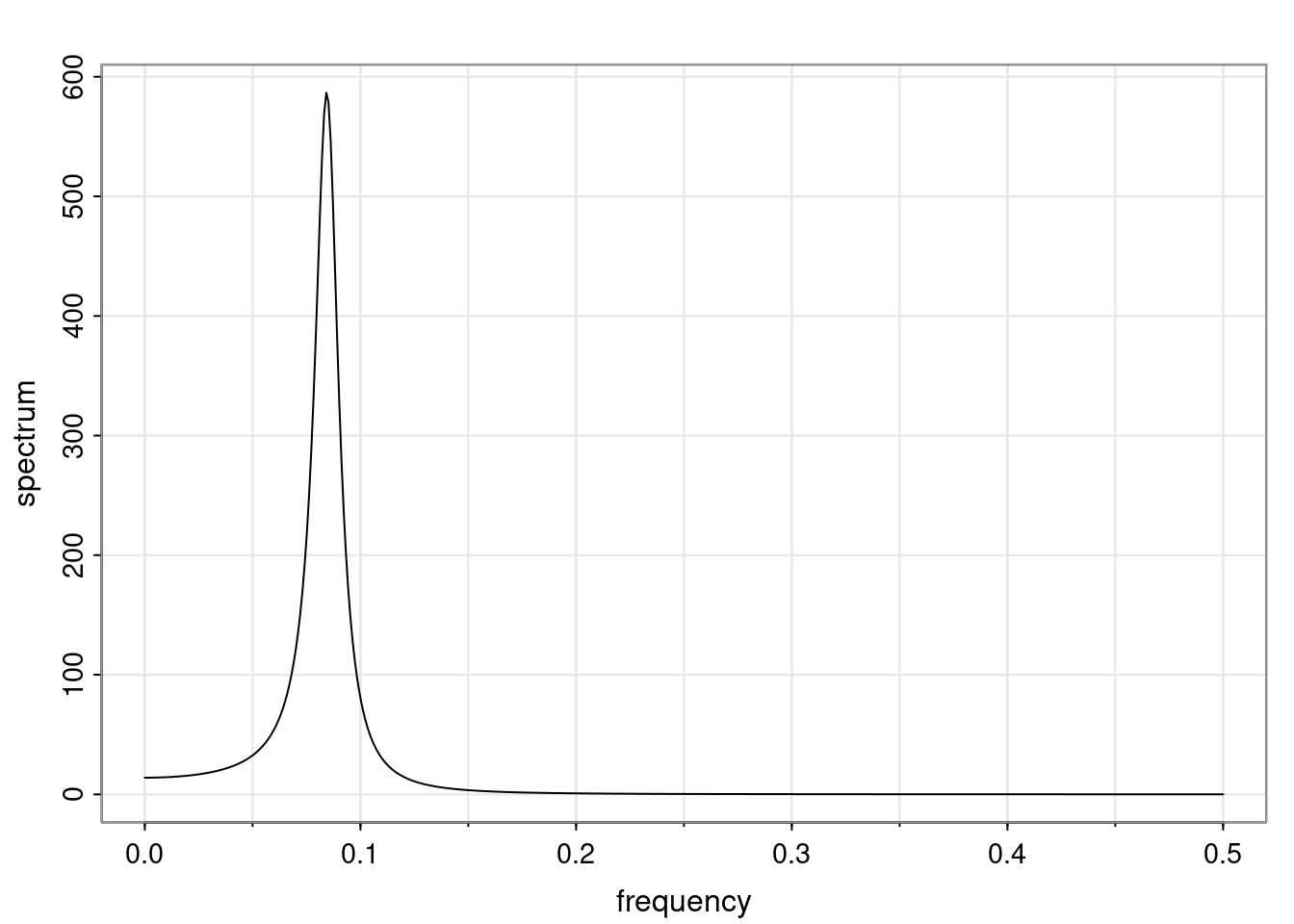
par(mfrow = c(1, 1))
#result_MLE=arma.spec(ar=phi_MLE, var.noise = s2, log='yes',main = '')
result_MLE=arma.spec(ar=phi_MLE, var.noise = s2, main = '')

Code
freq=result_MLE$freq
  
spec=matrix(0,nrow=n_sample,ncol=length(freq))

for (i in 1:n_sample){
result=arma.spec(ar=phi_sample[i,], var.noise = v_sample[i],# log='yes',
                 main = '')
spec[i,]=result$spec
}

Code
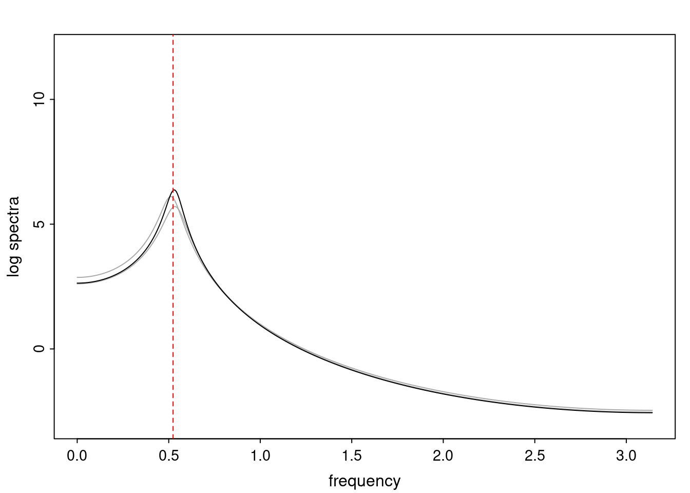
plot(2*pi*freq,log(spec[1,]),type='l',ylim=c(-3,12),ylab="log spectra",
     xlab="frequency",col=0)
#for (i in 1:n_sample){
for (i in 1:2){
lines(2*pi*freq,log(spec[i,]),col='darkgray')
}
lines(2*pi*freq,log(result_MLE$spec))
abline(v=2*pi/12,lty=2,col='red')

Quiz: Spectral representation of the AR(p)

Omitted due to Coursera’s Honor Code
Graded Assignment: Bayesian analysis of an EEG dataset using an AR(p)

The dataset below corresponds to a portion of an electroencephalogram (EEG) recorded in a particular location on the scalp of an individual. The original EEG dataset was originally recorded at 256Hz but was then subsampled every sixth observations, so the resulting sampling rate is about 42.7 observations per second. The dataset below has 400 observations corresponding approximately to 9.36 seconds.

You will use an AR(8) to model this dataset and obtain maximum likelihood estimation and Bayesian inference for the parameters of the model. For this you will need to do the following:

  1. Download the dataset, and plot it in R. Upload a picture of your graph displaying the data and comment on the features of the data. Does it present any trends or quasi-periodic behavior?

  2. Modify the code below to obtain the maximum likelihood estimators (MLEs) for the AR coefficients under the conditional likelihood. For this you will assume an autoregressive model of order p=8. The parameters of the model are \phi=(\phi_1, \ldots \phi_8)' snf v. You will compute the MLE of \phi denoted as \hat\phi. ​

  3. Obtain an unbiased estimator for the observational variance of the AR(8). You will compute the unbiased estimator for v denoted as s^2.

  4. Modify the code below to obtain 500 samples from the posterior distribution of the parameters \phi=(\phi_1, \ldots \phi_8)' and v under the conditional likelihood and the reference prior. You will assume an autoregressive model of order v. Once you obtain samples from the posterior distribution you will compute the posterior means of \phi and v, denoted as \hat\phi. and \hat v, respectively.

Modify the code below to use the function polyroot and obtain the moduli and periods of the reciprocal roots of the AR polynomial evaluated at the posterior mean \hat\phi.

Code
set.seed(2021)
r=0.95
lambda=12 
phi=numeric(2) 
phi[1]=2*r*cos(2*pi/lambda) 
phi[2]=-r^2
sd=1 # innovation standard deviation
T=300 # number of time points
# generate stationary AR(2) process
yt=arima.sim(n = T, model = list(ar = phi), sd = sd) 
par(mfrow=c(1,1))
plot(yt)

Code
## Case 1: Conditional likelihood
p=2
y=rev(yt[(p+1):T]) # response
X=t(matrix(yt[rev(rep((1:p),T-p)+rep((0:(T-p-1)),rep(p,T-p)))],p,T-p));
XtX=t(X)%*%X
XtX_inv=solve(XtX)
phi_MLE=XtX_inv%*%t(X)%*%y # MLE for phi
s2=sum((y - X%*%phi_MLE)^2)/(length(y) - p) #unbiased estimate for v

cat("\n MLE of conditional likelihood for phi: ", phi_MLE, "\n",
    "Estimate for v: ", s2, "\n")

 MLE of conditional likelihood for phi:  1.65272 -0.9189823 
 Estimate for v:  0.9901292 
Code
#####################################################################################
##  AR(2) case 
### Posterior inference, conditional likelihood + reference prior via 
### direct sampling                 
#####################################################################################

n_sample=1000 # posterior sample size
library(MASS)

## step 1: sample v from inverse gamma distribution
v_sample=1/rgamma(n_sample, (T-2*p)/2, sum((y-X%*%phi_MLE)^2)/2)

## step 2: sample phi conditional on v from normal distribution
phi_sample=matrix(0, nrow = n_sample, ncol = p)
for(i in 1:n_sample){
  phi_sample[i, ]=mvrnorm(1,phi_MLE,Sigma=v_sample[i]*XtX_inv)
}

## plot histogram of posterior samples of phi and nu
par(mfrow = c(1, 3), cex.lab = 1.3)
for(i in 1:2){
  hist(phi_sample[, i], xlab = bquote(phi), 
       main = bquote("Histogram of "~phi[.(i)]))
  abline(v = phi[i], col = 'red')
}

hist(v_sample, xlab = bquote(nu), main = bquote("Histogram of "~v))
abline(v = sd, col = 'red')

ARIMA processes (Reading)

ARMA Model Definition

A time series process is a zero-mean autoregressive moving average process if it is given by

y_t = \textcolor{red} {\underbrace{\sum_{i=1}^{p} \phi_i y_{t-i}}_{AR(P)}} + \textcolor{blue}{\underbrace{\sum_{j=1}^{q} \theta_j \epsilon_{t-j}}_{MA(Q)}} + \epsilon_t \qquad \text{(ARMA(p, q))} \tag{6}

with \epsilon_t \sim N(0, v).

  • For q = 0, we get an AR(p) process.
  • For p = 0, we get a MA(q) i.e. moving average process of order q.

Next we will define the notions of stability and invertibility of an ARMA process.

Stability Definition

An ARMA process is stable if the roots of the AR characteristic polynomial

stable

\Phi(u) = 1 - \phi_1 u - \phi_2 u^2 - \ldots - \phi_p u^p

lie outside the unit circle, i.e., for all u such that \Phi(u) = 0, |u| > 1.

Equivalently, this happens when the reciprocal roots of the AR polynomial have moduli smaller than 1.

This condition implies stationarity.

Invertible ARMA Definition

An ARMA process is invertible if the roots of the MA characteristic polynomial given by

invertible

\Theta(u) = 1 + \theta_1 u + \ldots + \theta_q u^q,

lie outside the unit circle.

Note that \Phi(B) y_t = \Theta(B) \epsilon_t.

  • When an ARMA process is stable, it can be written as an infinite order moving average process.

  • When an ARMA process is invertible, it can be written as an infinite order autoregressive process.

ARIMA Processes

An autoregressive integrated moving average process with orders p, d, and q is a process that can be written as

(1 - B)^d y_t = \sum_{i=1}^{p} \phi_i y_{t-i} + \sum_{j=1}^{q} \theta_j \epsilon_{t-j} + \epsilon_t,

in other words, y_t follows an ARIMA(p, d, q) if the d difference of y_t follows an ARMA(p, q).

Estimation in ARIMA processes can be done via least squares, maximum likelihood, and also in a Bayesian way. We will not discuss Bayesian estimation of ARIMA processes in this course.

Spectral Density of ARMA Processes

For a given AR(p) process with AR coefficients \phi_1, \dots, \phi_p and variance v, we can obtain its spectral density as

f(\omega) = \frac{v}{2\pi |\Phi(e^{-i\omega})|^2} = \frac{v}{2\pi |1 - \phi_1 e^{-i\omega} - \ldots - \phi_p e^{-ip\omega}|^2},

with \omega a frequency in (0, \pi).

The spectral density provides a frequency-domain representation of the process that is appealing because of its interpretability.

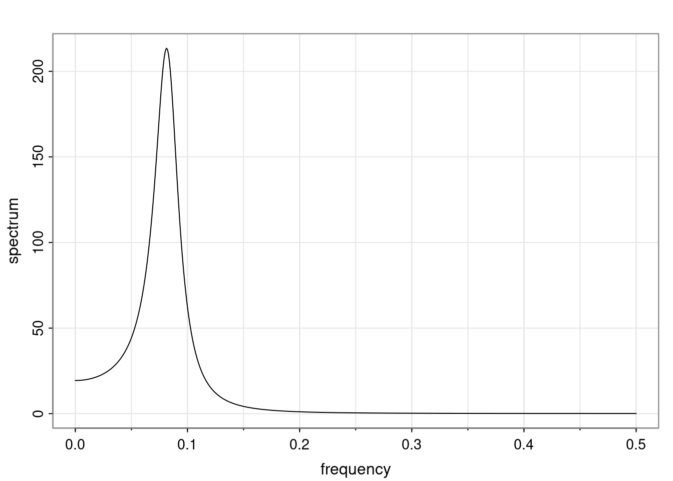
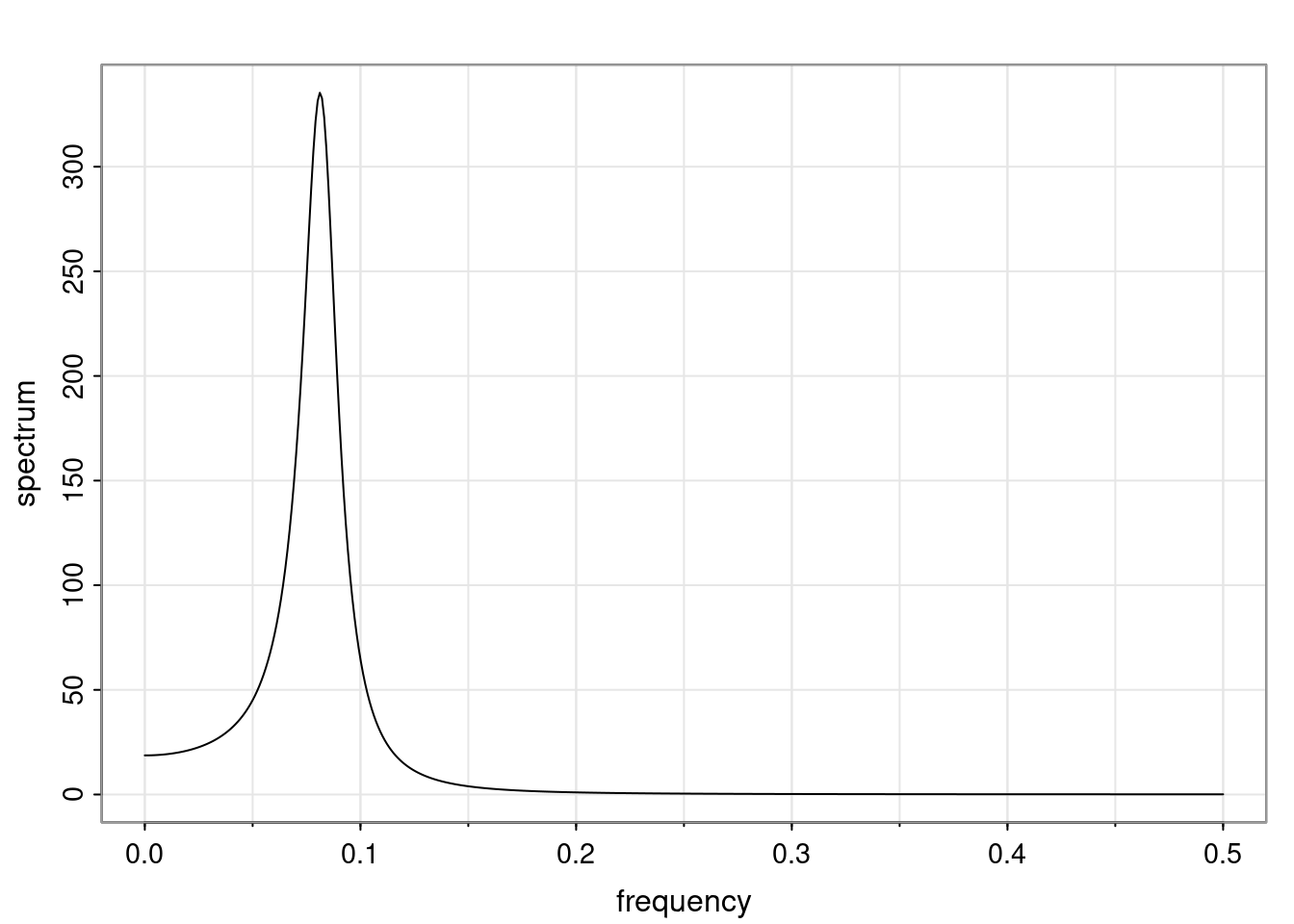
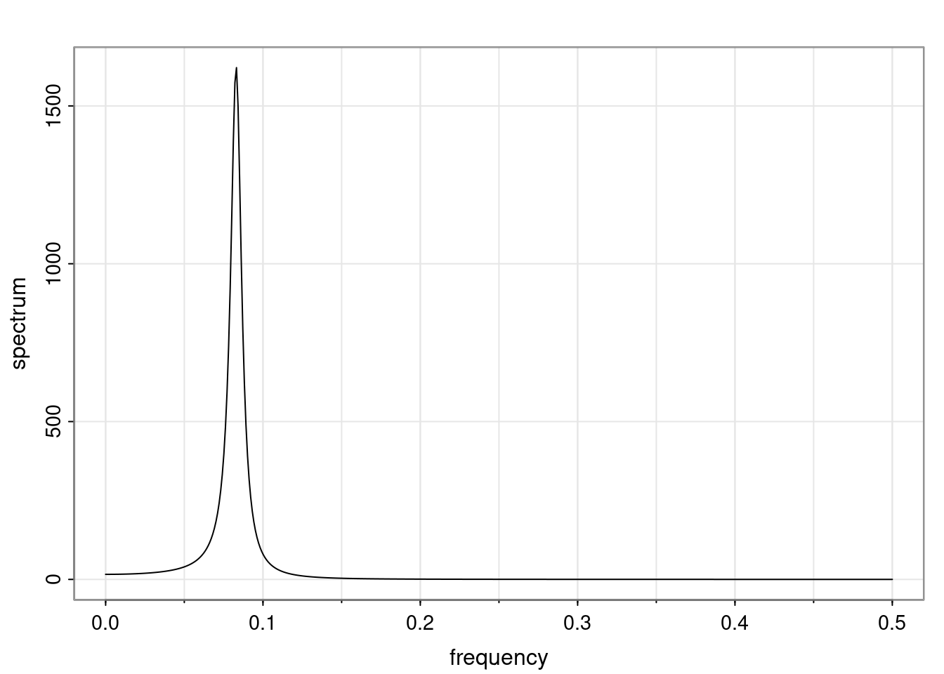
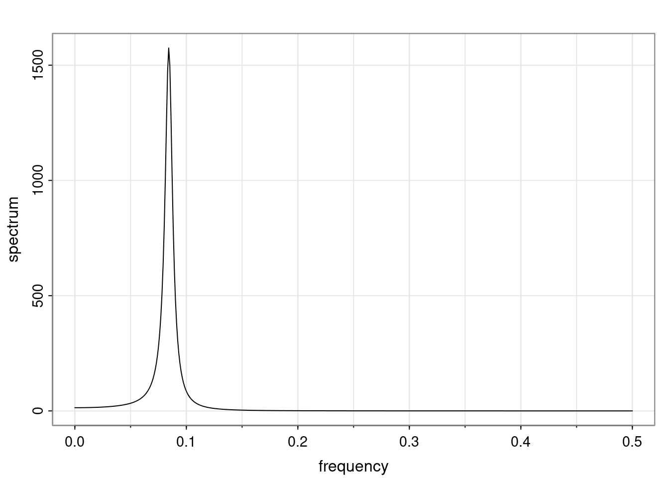
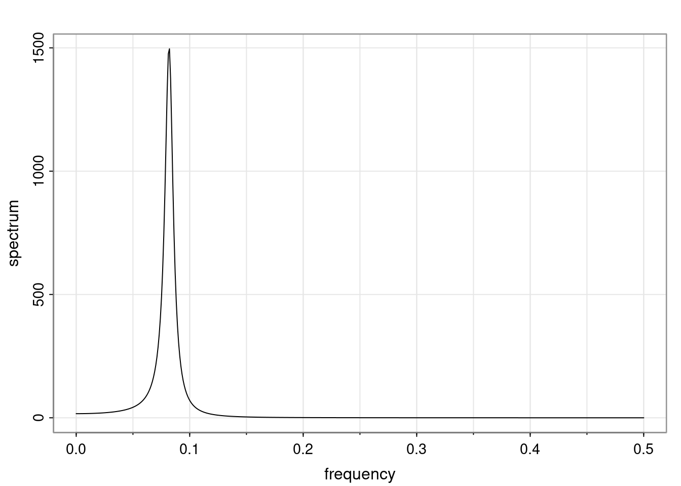
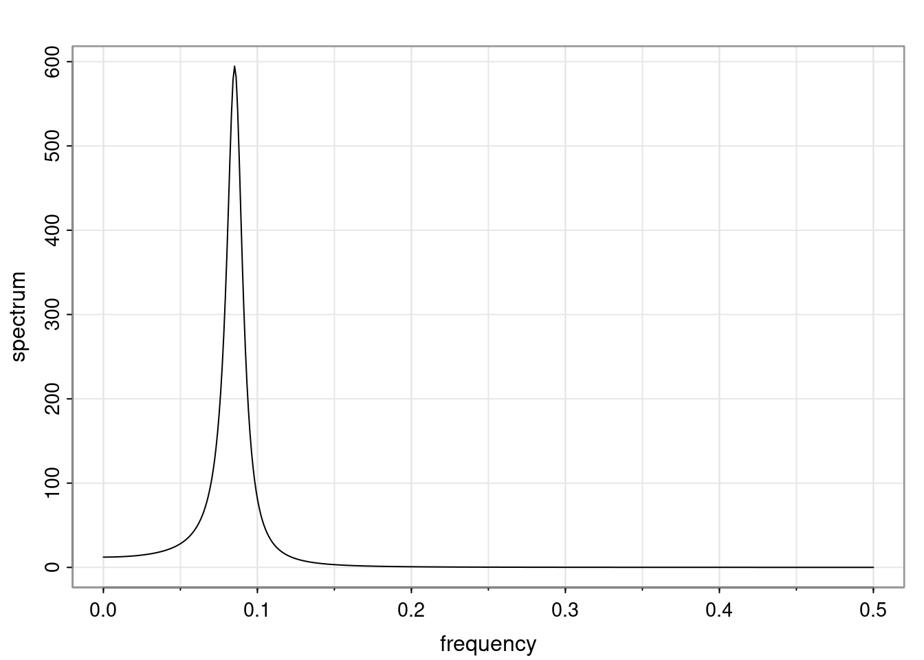
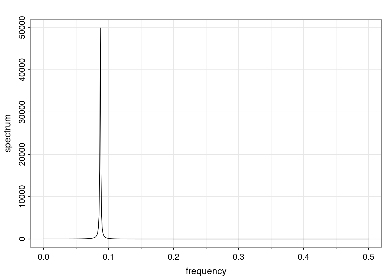
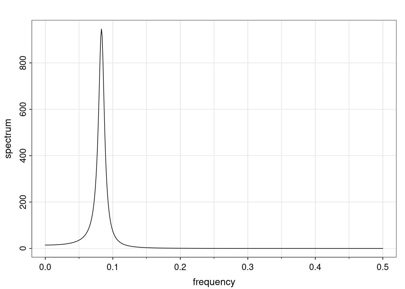
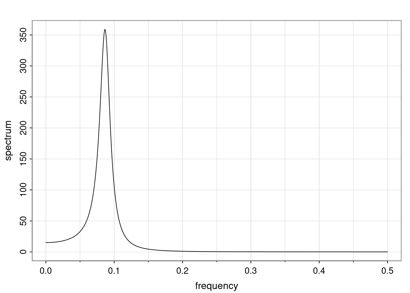
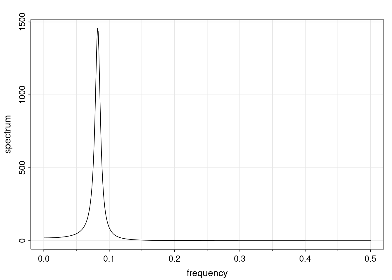
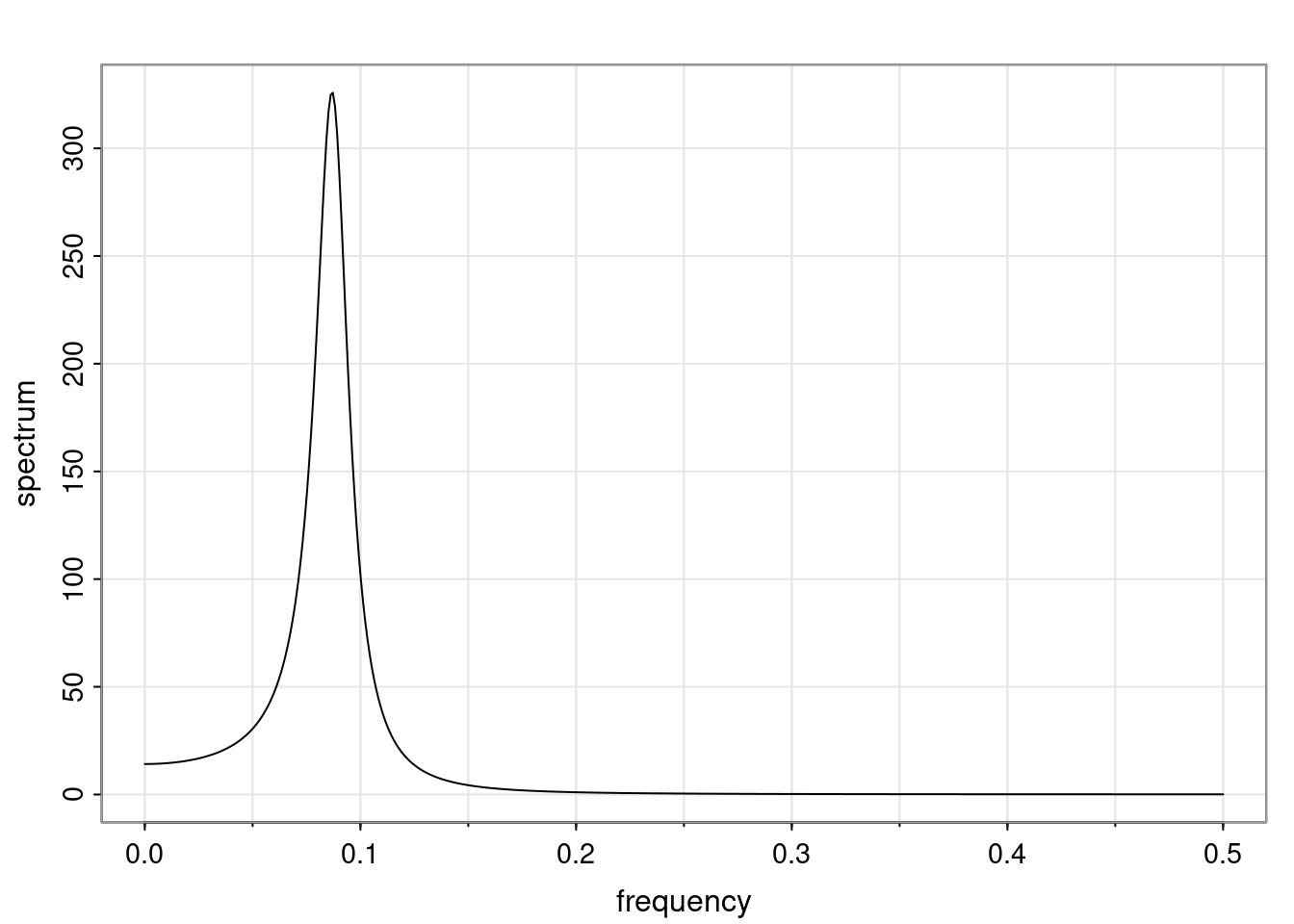
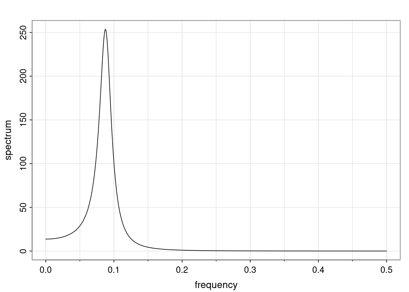
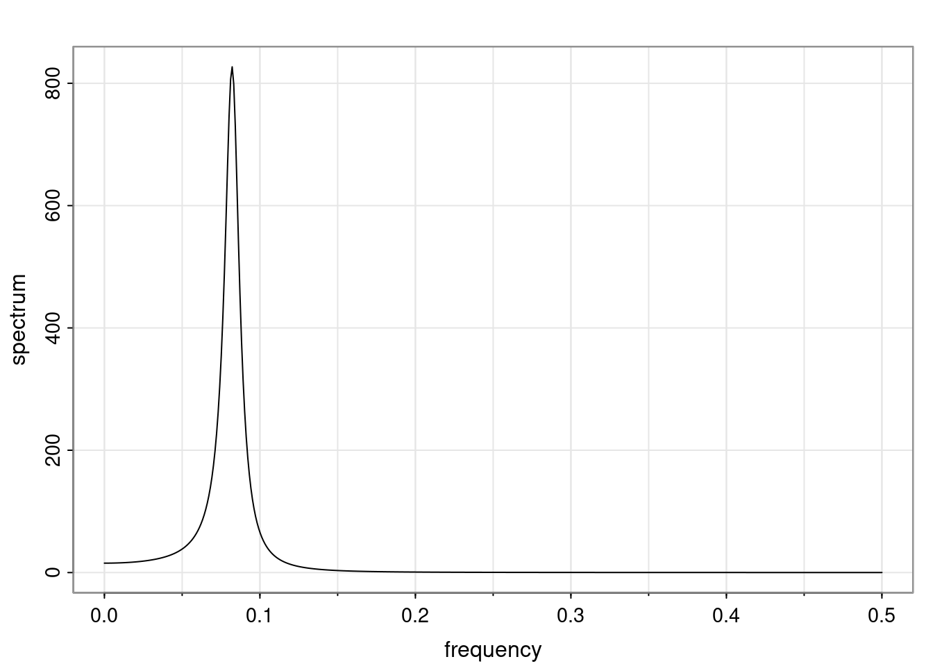
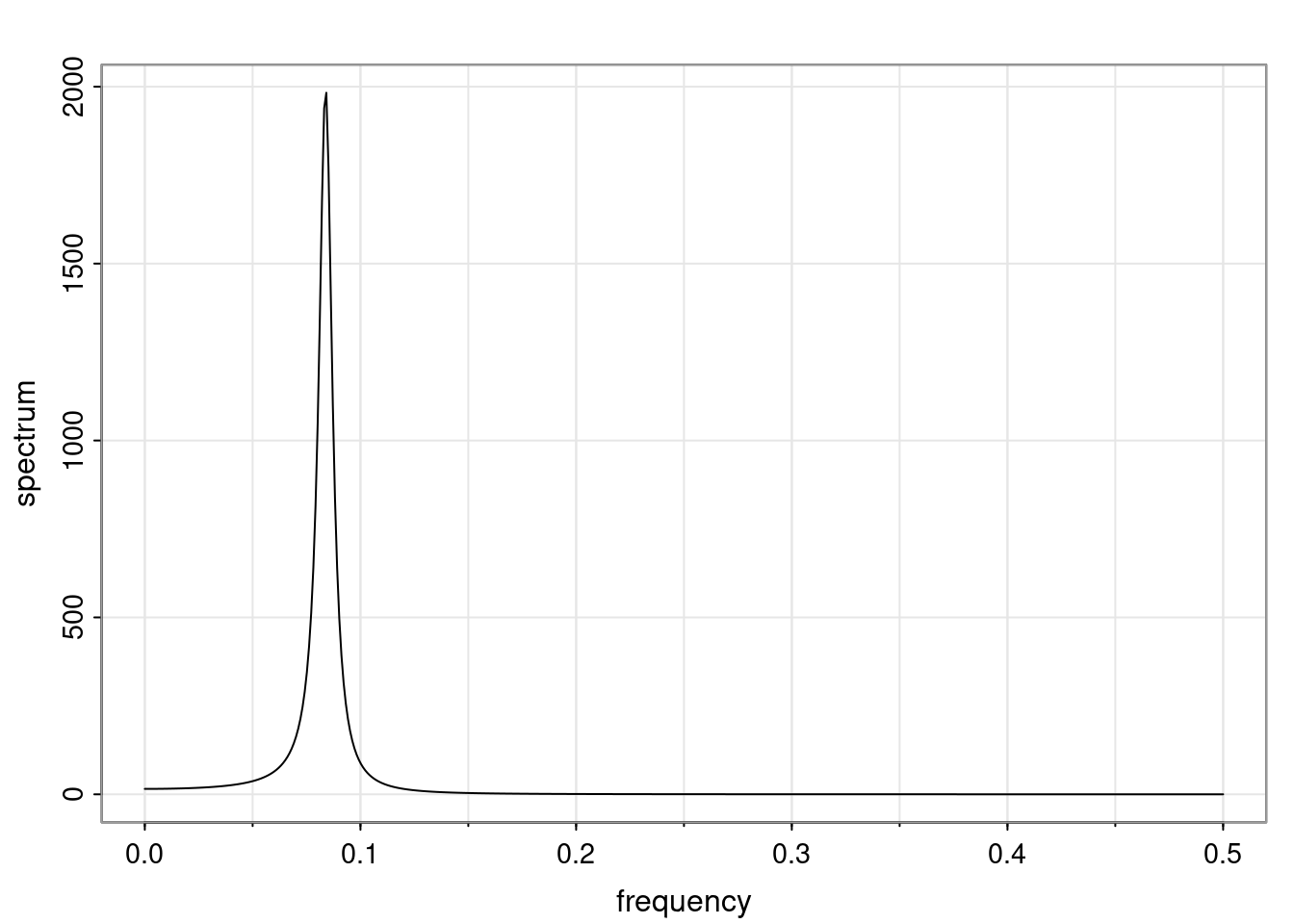
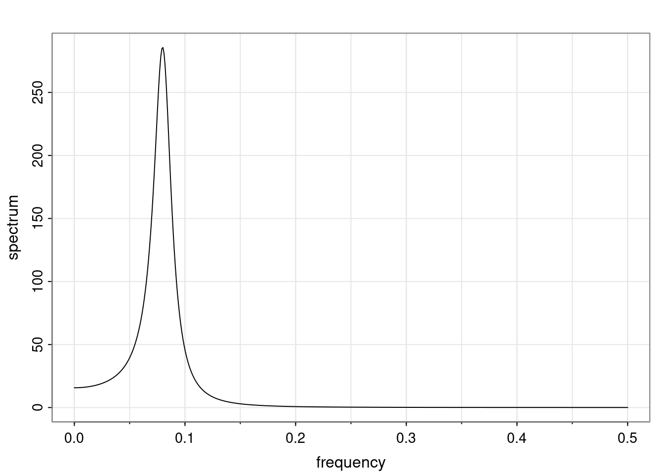
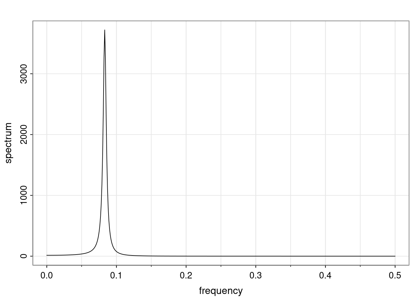
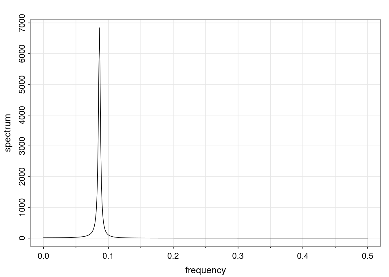
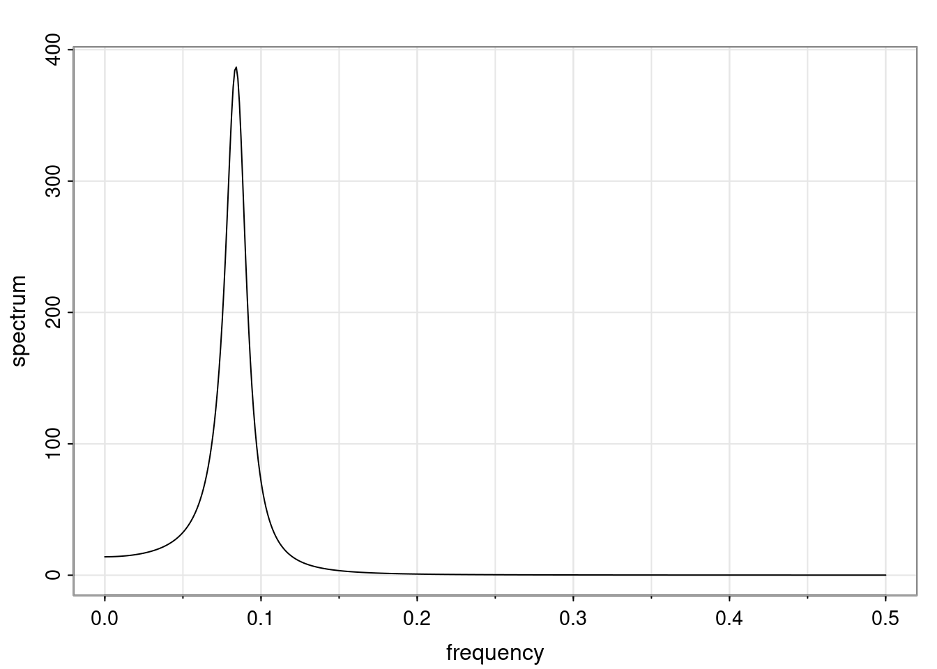
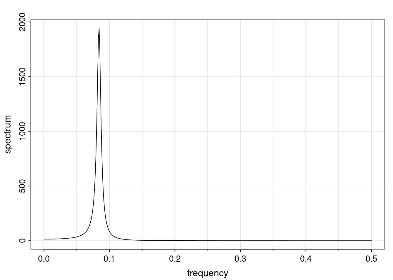
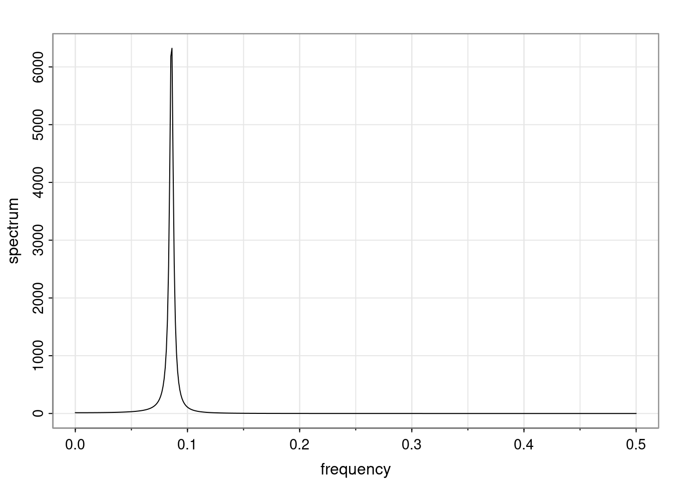
For instance, an AR(2) process that has one pair of complex-valued reciprocal roots with modulus 0.7 and a period of \lambda = 12, will show a mode in the spectral density located at a frequency of 2\pi/12. If we keep the period of the process at the same value of 12 but increase its modulus to 0.95, the spectral density will continue to show a mode at 2\pi/12, but the value of f(2\pi/12) will be higher, indicating a more persistent quasi-periodic behavior.

Similarly, we can obtain the spectral density of an ARMA process with AR characteristic polynomial \Phi(u) = 1 - \phi_1 u - \ldots - \phi_p u^p and MA characteristic polynomial \Theta(u) = 1 + \theta_1 u + \ldots + \theta_q u^q, and variance v as

f(\omega) = \frac{v}{2\pi} \frac{|\Theta(e^{-i\omega})|^2}{|\Phi(e^{-i\omega})|^2}.

Note that if we have posterior estimates or posterior samples of the AR/ARMA coefficients and the variance v, we can obtain samples from the spectral density of AR/ARMA processes using the equations above.

Reuse

CC SA BY-NC-ND

Citation

BibTeX citation:
@online{bochman2024,
  author = {Bochman, Oren},
  title = {Week 2: {The} {AR(p)} Process},
  date = {2024-10-24},
  url = {https://orenbochman.github.io/notes/bayesian-ts/module2.html},
  langid = {en}
}
For attribution, please cite this work as:
Bochman, Oren. 2024. “Week 2: The AR(p) Process.” October 24, 2024. https://orenbochman.github.io/notes/bayesian-ts/module2.html.