I decided to migrate some material that is auxilary to the course:
- An overview of the course.
- A review of some mathematical and statistical results used in the course.
- A bibliography of books I found useful in the course.
- A Feynman notebook for the course - is now in a separate notebook.
Course Card
- Course: Bayesian Statistics: Time Series
- Offered by: University of California, Santa Cruz
- Instructor: Raquel Prado
- Certificate: Yes
- Level: Graduate
- Commitment: 4 weeks of study, 3-4 hours/week
Overview of the course
This course seems very similar to classic basic time series course without the Bayesian part. (AR, MA, ARMA, ARIMA, SARIMA, DLM etc.)
One of the questions I had when I started this course was what is the difference between a Bayesian approach to time series analysis and a classical approach. The following is a summary of what I found:
The Bayesian approach presents primarily in:
- Sections on Bayesian inference where we do inference on the parameters of the models.
- Bayesian prediction unlike an MLE prediction is a distribution of predictions not just a point estimate, and therefore is useful for quantifying uncertainty.
- We also cover some material on model selection - this again is where the Bayesian approach to optimization presents more powerful tools than the classical approach.
- When we want to quantify the uncertainty in our model we have four sources of uncertainty:
- Uncertainty due to using the correct model (structure).
- I consider this is an epistemic uncertainty -
- One could reduce it by collecting more data, then applying the Bayesian model selection to choose the best model.
- Uncertainty due to the estimation of the model parameters. This is an epistemic uncertainty - we can reduce it by collecting more data reducing the plausible intervals for these parameters under the bayesian approach.
- Uncertainty due to random shocks \epsilon_t. for the period being predicted. This is an aleatory uncertainty.
- Uncertainty in the forecasted values X_{t+h} Items 2-3 can be quantified using a plausible interval in the Bayesian approach and as we predict further into the future the interval will grow.
- Uncertainty due to using the correct model (structure).
- Model selection is a big part of the Bayesian approach. We can use the DIC, WAIC, and LOO to compare models.
- The book by Professor Prado is very comprehensive and covers plenty of additional models and references lots of recent research. These including VAR, VARMA models, Kalman filters, SMC/Particle filters, etc. These are useful for the continuous control flavours of RL. But you will need to learn it on your own.
- In the capstone project that is the next course in the specialization the teacher adds another layer of sophistication by introducing mixtures of TS models.
- However unlike some courses I took we dive deep enough and get sufficient examples to understand how to put all the bits together into more sophisticated time series models.
Mathematical Review
There is a issues with mathematics most of the results and techniques are so rarely useful that students will soon forget most but a few very useful results. Having a good memory is a great asset in mathematics but is rarely enough. I like to review some mathematical results from my undergraduate days evey five years or so. This helps me keep many of the results fresh in my mind and also makes reading new mathematics easier. Fundamentals in mathematics can fo a very long way. This is material from topology, determinants and solving linear equations, numerical methods for decomposing matrices, and so on. Definions of certain groups.
One reason this and other baysian courses and books can be challenging and even overwhlming is that they can use lots of mathematics. This can range from high school material like complex numbers and quadratics formulas to intermediate results like finding root of characteristic polynomials, eigenvalues, Topelitz matrices, jordan forms, and advanced topics like the Durbin-Levinson recursion and certain results from functional analysis theory.
Note that I have not even touched on probability and statistics in that list.
Rather than complain I see this as an opportunity to review/learn some mathematics and statistics that can be useful to a data scientist. During my last sting in Data science I often was able to write formulas but more often then not felt that I lacked sufficent mathematical tools to manipulate them to get the kind of results I wanted. Rather then learning lots of mathematics I wanted to find the most practical and useful results for wrangling maths. When I was a physics undergraduate these might be trigonometric identities, completing the square, being familier with many integrals and taylor or macclaurin series approximations and a few useful inequalities occasionally we use l’Hopital’s rule. Familiarity with some ODEs was also greatly beneficial as therse come up in many physical models. Later on hermitian and unitary matrices, fourier expansions, spectral theory, and some results from functional analysis were useful.
For statistics we have the variants of the law of large numbers and the central limit theorem, convergence theorems, manupulations of the normal distribution, linear properties of expectation can get you along way. But you have to remeber lots of definitions and there are lots of results and theorems that seem to be stepping stones to other results rather than any practical use.
On the other hand congugacy of certain distributions as demonsterated by herbert lee and other instructors in this specilization are often very challenging. Charts of Conergence of distributions to other distributions under certain conditions are neat but. There is Hodfing’s inequality and the Markov inequality which can be useful but like most results in mathematics I never had a where they might be used. Then there are certain results - convergence of Markov chains, doubly stochastic matrices. De Finetti’s theorem in statistics.
I have found that the more I learn the more I can understand and appreciate the material.
- The autoregressive process gives rise to Toeplitz matrices which can be solved using the Durbin-Levinson recursion mentioned many times in the course.
- Durbin-Levinson recursion - is an advanced topic not covered in Numerical Analysis courses or Algebra courses I took.
- To use it with time series we also need to understand the Yule-Walker equations.
- ar(p) require some linear algebra concepts like eigenvalues and Eigenvectors, and characteristic polynomials.
- The AR(p) the Wold decomposition theorem to get to the infinite order moving average representation and this is not a result I recall learning in my functional analysis course. We also use some complex numbers and Fourier analysis and spectral density functions.
Summarize some of the extra curricular material I found useful in the course.
Complex Numbers (Review)
When we wish to find the roots of real valued polynomials we will often encounter complex numbers. In this course such polynomials arise naturally in the characteristic polynomials of AR(p) processes.
We will need the polar form of complex numbers to represent some variants of AR(p) process.
The numbers in the Complex field z \in \mathbb{C} numbers are numbers that can be expressed in the form z = a + bi, where a,b\in\mathbb{R} and i is the imaginary unit. The imaginary unit i is defined as the square root of -1. Complex numbers can be added, subtracted, multiplied, and divided just like real numbers.
The complex conjugate of a complex number z = a + bi is denoted by \bar{z} = a - bi. The magnitude of a complex number z = a + bi is denoted by |z| = \sqrt{a^2 + b^2}. This is sometimes called the modulus of the complex number in this course. The argument of a complex number z = a + bi is denoted by \text{arg}(z) = \tan^{-1}(b/a). The polar form of a complex number is given by z = r e^{i \theta}, where r = |z| and \theta = \text{arg}(z).
The polar form of a complex number is given by:
\begin{aligned} z &= \mid z\mid e^{i \theta} \\ &= r (\cos(\theta) + i \sin(\theta)) \end{aligned} \tag{1}
where:
- |z| is the magnitude of the complex number, i.e. the distance from the origin to the point in the complex plane.
- \theta is the angle of the complex number.
I think we will also need the unit roots.
Eigenvalues, Eigenvectors the characteristic polynomials and Unit roots
The Eigenvalues of a matrix are the roots of the characteristic polynomial of the matrix. The characteristic polynomial of a matrix A is defined as:
\begin{aligned} \text{det}(A - \lambda I) = 0 \end{aligned}
where \lambda is the Eigenvalue and I is the identity matrix. The eigenvectors of a matrix are the vectors that satisfy the equation:
\begin{aligned} A v = \lambda v \end{aligned}
where v is the eigenvector and \lambda is the eigenvalue. The eigenvalues and eigenvectors of a matrix are used in many applications in mathematics and physics, including the diagonalization of matrices, the solution of differential equations, and the analysis of dynamical systems.
Unit Roots
A unit root is a root of the characteristic polynomial of an autoregressive model that is equal to 1. The presence of a unit root in an autoregressive model indicates that the model is not stationary. The unit root test is a statistical test that is used to determine whether a time series is stationary or non-stationary. The unit root test is based on the null hypothesis that the time series has a unit root, and the alternative hypothesis that the time series is stationary. The unit root test is used to determine whether a time series is stationary or non-stationary, and is an important tool in time series analysis.
Spectral analysis (1898)
The power spectrum of a signal is the squared absolute value of its Fourier transform. If it is estimated from the discrete Fourier transform it is also called periodogram. Usually estimated using the a fast Fourier transform (FFT) algorithm.
Yule-Walker Equations (1932)
Durbin-Levinson recursion (Off-Course Reading)
Like me, you might be curious about the Durbin-Levinson recursion mentioned above. This is not covered in the course, and turned out to be an enigma wrapped in a mystery.
I present my finding in the note below - much of it is due to (Wikipedia contributors 2024b) and (Wikipedia contributors 2024a)
In (Yule 1927) and (Walker 1931), Yule and Walker proposed a method for estimating the parameters of an autoregressive model. The method is based on the Yule-Walker equations which are a set of linear equations that can be used to estimate the parameters of an autoregressive model.
Due to the autoregressive nature of the model, the equations are take a special form called a Toeplitz matrix. However at the time they probably had to use the numerically unstable Gauss-Jordan elimination to solve these equations which is O(n^3) in time complexity.
A decade or two later in (Levinson 1946) and (Durbin 1960) the authors came up for with a weakly stable yet more efficient algorithm for solving these autocorrelated system of equations which requires only O(n^2) in time complexity. Later their work was further refined in (Trench 1964) and (Zohar 1969) to just 3\times n^2 multiplication. A cursory search reveals that Toeplitz matrix inversion is still an area of active research with papers covering parallel algorithms and stability studies. Not surprising as man of the more interesting deep learning models, including LLMs are autoregressive.
So the Durbin-Levinson recursion is just an elegant bit of linear algebra for solving the Yule-Walker equations more efficiently.
Here is what I dug up:
Durbin-Levinson and the Yule-Walker equations (Off-Course Reading)
The Durbin-Levinson recursion is a method in linear algebra for computing the solution to an equation involving a Toeplitz matrix AKA a diagonal-constant matrix where descending diagonals are constant. The recursion runs in O(n^2) time rather then O(n^3) time required by Gauss-Jordan elimination.
The recursion can be used to compute the coefficients of the autoregressive model of a stationary time series. It is based on the Yule-Walker equations and is used to compute the PACF of a time series.
The Yule-Walker equations can be stated as follows for an AR(p) process:
\gamma_m = \sum_{k=1}^p \phi_k \gamma_{m-k} + \sigma_\epsilon^2\delta_{m,0} \qquad \text{(Yule-Walker equations)} \tag{2}
where:
- \gamma_m is the autocovariance function of the time series,
- \phi_k are the AR coefficients,
- \sigma_\epsilon^2 is the variance of the white noise process, and
- \delta_{m,0} is the Kronecker delta function.
when m=0 the equation simplifies to:
\gamma_0 = \sum_{k=1}^p \phi_k \gamma_{-k} + \sigma_\epsilon^2 \qquad \text{(Yule-Walker equations for m=0)} \tag{3}
for m > 0 the equation simplifies to:
\begin{bmatrix} \gamma_1 \newline \gamma_2 \newline \gamma_3 \newline \vdots \newline \gamma_p \newline \end{bmatrix} = \begin{bmatrix} \gamma_0 & \gamma_{-1} & \gamma_{-2} & \cdots \newline \gamma_1 & \gamma_0 & \gamma_{-1} & \cdots \newline \gamma_2 & \gamma_1 & \gamma_0 & \cdots \newline \vdots & \vdots & \vdots & \ddots \newline \gamma_{p-1} & \gamma_{p-2} & \gamma_{p-3} & \cdots \newline \end{bmatrix} \begin{bmatrix} \phi_{1} \newline \phi_{2} \newline \phi_{3} \newline \vdots \newline \phi_{p} \newline \end{bmatrix}
and since this matrix is Toeplitz, we can use Durbin-Levinson recursion to efficiently solve the system for \phi_k \forall k.
Once \{\phi_m ; m=1,2, \dots ,p \} are known, we can consider m=0 and solved for \sigma_\epsilon^2 by substituting the \phi_k into Equation 3 Yule-Walker equations.
Of course the Durbin-Levinson recursion is not the last word on solving this system of equations. There are today numerous improvements which are both faster and more numerically stable.
The Yule-Walker equations are a set of p linear equations in the p unknowns \phi_1, \phi_2, \ldots, \phi_p that can be used to estimate the parameters of an autoregressive model of order p. The Yule-Walker equations are derived by setting the sample autocorrelation function equal to the theoretical autocorrelation function of an AR(p) model and then solving for the unknown parameters. The Yule-Walker equations are given by:
\begin{aligned} \gamma(0) & = \phi_1 \gamma(1) + \phi_2 \gamma(2) + \ldots + \phi_p \gamma(p) \\ \gamma(1) & = \phi_1 \gamma(0) + \phi_2 \gamma(1) + \ldots + \phi_p \gamma(p-1) \\ \gamma(2) & = \phi_1 \gamma(1) + \phi_2 \gamma(0) + \ldots + \phi_p \gamma(p-2) \\ \vdots \\ \gamma(p) & = \phi_1 \gamma(p-1) + \phi_2 \gamma(p-2) + \ldots + \phi_p \gamma(0) \\ \end{aligned}
where \gamma(k) is the sample autocorrelation function at lag k. The Yule-Walker equations can be solved using matrix algebra to obtain the estimates of the AR parameters \phi_1, \phi_2, \ldots, \phi_p.
Wold’s theorem - (extra curricular) circa 1939
In the 1920 Yule and Eugen Slutsky were researching time series and they came up with two different ways to represent a time series.
Yule’s researches led to the notion of the autoregressive scheme. \begin{aligned} Y_{t} & = \sum _{j=1}^{p} \phi _{j} Y_{t-j} + u_{t} \end{aligned} \tag{4}
Slutsky’s researches led to the notion of a moving average scheme. \begin{aligned} Y_{t} & =\sum _{j=0}^{q} \theta _{j} u_{t-j} \end{aligned} \tag{5}
we can use the two schemes together and get the ARMA(p,q) model:
\begin{aligned} Y_{t} & = \sum _{j=1}^{p} \phi _{j} Y_{t-j} + u_{t} + \sum _{j=0}^{q} \theta _{j} u_{t-j} \end{aligned} \tag{6}
where:
The following is extracted from: the wikipedia at https://en.wikipedia.org/wiki/Wold%27s_theorem
Wold’s decomposition AKA called the Wold representation theorem states that:
Every covariance-stationary time series Y_{t} can be written as the sum of two time series, one deterministic and one stochastic.
Formally:
\begin{aligned} Y_{t} & =\sum _{j=0}^{\infty } \underbrace{b_{j}\epsilon _{t-j}}_{\text{stochastic}} + \underbrace{\eta _{t}}_{\text{deterministic}} \\ &= \sum _{j=0}^{\infty } b_{j}\epsilon _{t-j} + \phi_{j} y_{t-j} \end{aligned}
where:
- {Y_{t}} is the time series being considered,
- {\epsilon _{t}} is an white noise sequence called innovation process that acts as an input to the linear filter {\{b_{j}\}}.
- {b} is the possibly infinite vector of moving average weights (coefficients or parameters)
- {\eta _{t}} is a “deterministic” time series, in the sense that it is completely determined as a linear combination of its past values It may include “deterministic terms” like sine/cosine waves of {t}, but it is a stochastic process and it is also covariance-stationary, it cannot be an arbitrary deterministic process that violates stationarity.
The moving average coefficients have these properties:
- Stable, that is, square summable \sum _{j=1}^{\infty } \mid b_{j}|^{2} < \infty
- Causal (i.e. there are no terms with j < 0)
- Minimum delay
- Constant (b_j independent of t)
- It is conventional to define b_0=1
Any stationary process has this seemingly special representation. Not only is the existence of such a simple linear and exact representation remarkable, but even more so is the special nature of the moving average model.
This result is used without stating its name in the course when we are show the AR(p) representation in terms of moving averages.
Kalman Filter (1960)
\begin{aligned} x_{t} & = F_{t} x_{t-1} + G_{t} u_{t} + w_{t} && \text{(transition equation)} \\ y_{t} & = H_{t} x_{t} + v_{t} && \text{(observation equation)} \end{aligned} \tag{7}
where:
- x_{t} is the state vector at time t,
- F_{t} is the state transition matrix,
- G_{t} is the control input matrix,
- u_{t} is the control vector,
- w_{t} is the process noise vector,
- y_{t} is the observation vector at time t,
- H_{t} is the observation matrix,
- v_{t} is the observation noise vector.
The Kalman filter is a recursive algorithm that estimates the state of a linear dynamic system from a series of noisy observations. The Kalman filter is based on a linear dynamical system model that is defined by two equations: the state transition equation and the observation equation. The state transition equation describes how the state of the system evolves over time, while the observation equation describes how the observations are generated from the state of the system. The Kalman filter uses these two equations to estimate the state of the system at each time step, based on the observations received up to that time step. This could be implemented in real time in the 1960s and was used in the Apollo missions.
The Extended Kalman Filter (EKF) is an extension of the Kalman filter that can be used to estimate the state of a nonlinear dynamic system. The EKF linearizes the nonlinear system model at each time step and then applies the Kalman filter to the linearized system. The EKF is an approximation to the true nonlinear system, and its accuracy depends on how well the linearized system approximates the true system.
Box Jenkins Method (1970)
A five step process for identifying, selecting and assessing ARMA (and similar) models.
- There are three courses on Stochastic Processes on MIT OCW that I found useful:
- Introduction to Stochastic Processes
- Discrete Stochastic Processes
- has kecture videos and notes
- poisson processes
- Advanced Stochastic Processes
- martingales
- ito calculus
Bayesian Time Series Bibliography
We start with some books from the course, I collected here both the recommended books and some others that I found useful.
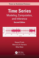
Time Series: Modeling, Computation, and Inference
c.f. (Prado, Ferreira, and West 2023)
- Title:Time Series: Modeling, Computation, and Inference
- ISBN:9781032040042, 1032040041
- Page count:452
- Published:September 2023
- Format:Paperback
- Publisher:CRC Press
- Authors: Raquel Prado, Marco A. R. Ferreira, Mike West
(Prado, Ferreira, and West 2023) “Time Series: Modeling, Computation, and Inference” by course instructor Raquel Prado. This book, now in its second edition is a comprehensive introduction to time series analysis and covers a wide range of topics in time series modeling, computation, and inference. The book is suitable for graduate students and researchers in statistics, computer science, and related fields.
While learning this course I found some of the material harder to follow than I expected. The books helped to clarify definitions and so on however the book is
rather comprehensive and mathematically advanced unlike some other books on statistics.
The teacher frequently point out that many aspects of Times series and are beyond the scope of the course. Yet this book covers much more ground like unequaly spaced time series and vector valued time series.
For example we look at EKG data which the authors have been working on for years. However we look at it in this course in terms of a univariate time series while in reality EKG is usually sampled at 12 sites simultaneously yielding a multi-variate time series.
Once this course is done I will probably want to dive deeper into the subject and try to devote more time to other models in the book.
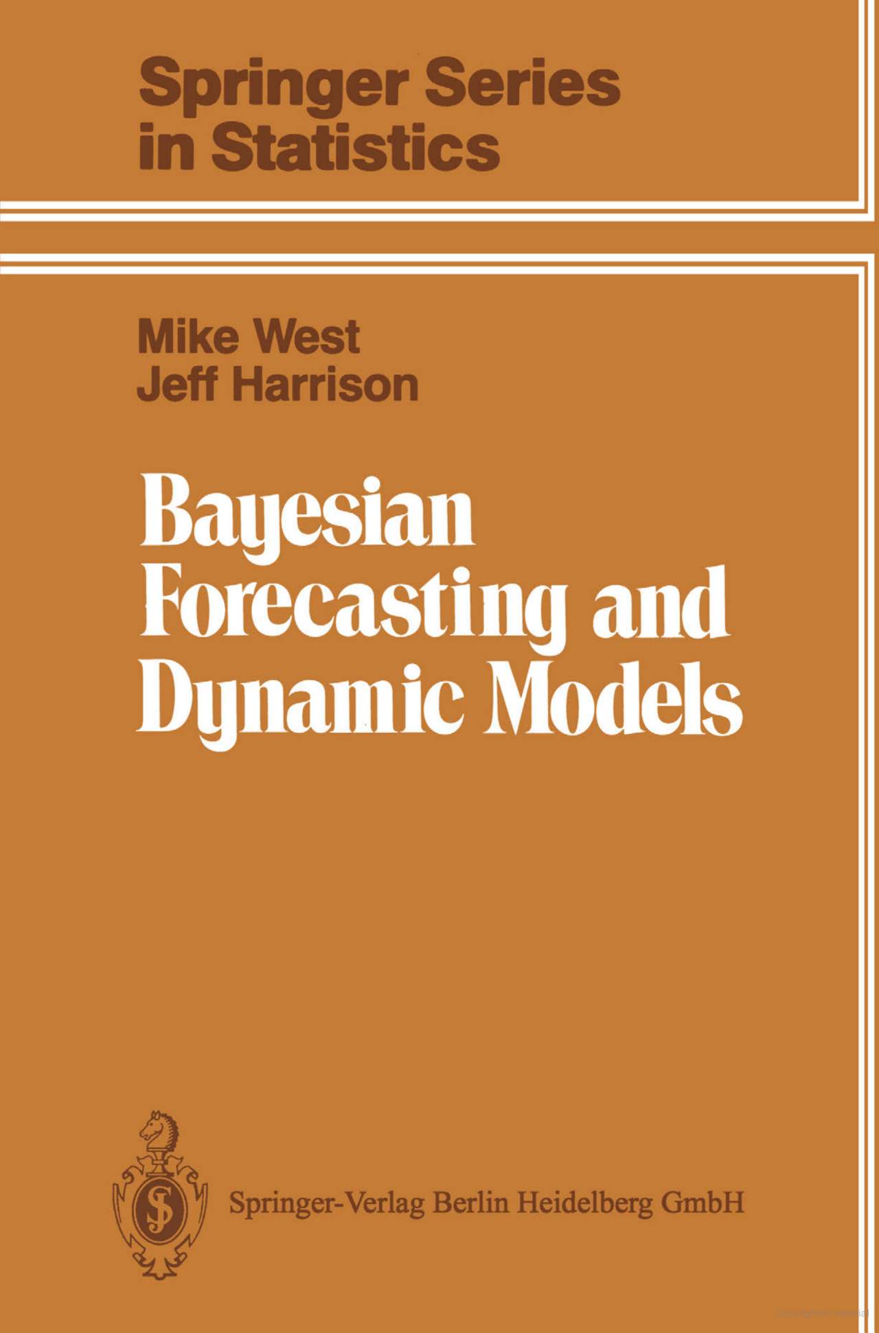
Bayesian Forecasting and Dynamic Models
c.f. (West and Harrison 2013)
- Title:Bayesian Forecasting and Dynamic Models
- ISBN:9781475770971, 1475770979
- Page count:682
- Published:March 17, 2013
- Format:Paperback
- Publisher:Springer New York
- Author:Mike West, Jeff Harrison
(West and Harrison 2013) “Bayesian Forecasting and Dynamic Models” by Mike West and Jeff Harrison. This book is a classic text on Bayesian statistics and covers a wide range of topics in Bayesian forecasting and dynamic models. The following is the description from the publisher:
The use of dynamic models in the forecasting of time series data has a long history, with the development of autoregressive integrated moving average (ARIMA) models and state space models. However, the use of Bayesian methods in the development of dynamic models is a relatively recent development. This book provides a comprehensive introduction to the use of Bayesian methods in the development of dynamic models for forecasting time series data. The book covers a wide range of topics, including the use of dynamic models in the analysis of time series data, the use of Bayesian methods in the development of dynamic models, and the use of dynamic models in the forecasting of time series data.
- Audience: The book is suitable for graduate students and researchers in statistics, computer science, and related fields.
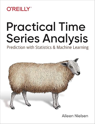
Practical Time Series Analysis
c.f. (Nielsen 2019)
Title:Practical Time Series Analysis: Prediction with Statistics and Machine Learning
ISBN:1492041602, 9781492041603
Page count:504
Published:2019
Format:Paperback
Publisher:O’Reilly Media, Inc.
(Nielsen 2019) “Practical Time Series Analysis: Prediction with Statistics and Machine Learning” by Aileen Nielsen. Is a good resource for parctionars getting started with time series analysis. I also recommend any videos by Aileen Nielsen on the subject.
Practical Times Series Analysis by Aileen Nielsen is a good book for beginners. It is a practical guide to time series analysis and covers a wide range of topics in time series modeling, computation, and inference. The book is suitable for beginners in statistics, computer science, and related fields.
Time series data analysis is increasingly important due to the massive production of such data through the internet of things, the digitalization of healthcare, and the rise of smart cities. As continuous monitoring and data collection become more common, the need for competent time series analysis with both statistical and machine learning techniques will increase.
Covering innovations in time series data analysis and use cases from the real world, this practical guide will help you solve the most common data engineering and analysis challenges in time series, using both traditional statistical and modern machine learning techniques. Author Aileen Nielsen offers an accessible, well-rounded introduction to time series in both R and Python that will have data scientists, software engineers, and researchers up and running quickly.
You’ll get the guidance you need to confidently:
- Find and wrangle time series data
- Undertake exploratory time series data analysis
- Store temporal data
- Simulate time series data
- Generate and select features for a time series
- Measure error
- Forecast and classify time series with machine or deep learning
- Evaluate accuracy and performance
“Machine Learning: A Bayesian and Optimization Perspective” by Sergios Theodoridis.
c.f. (Theodoridis 2015)
- Title:Machine Learning: A Bayesian and Optimization Perspective
- ISBN:0128015225, 9780128015223
- Page count:1062
- Published:2015
- Format:Hardcover
- Publisher:Academic Press
- Authors: Sergios Theodoridis
I came across this book while looking into the Durban-Levinson recursion and the Yule-Walker equations. So far I haven’t had time to read it but it looks like a good book on machine learning. The following is the description from the publisher:
This tutorial text gives a unifying perspective on machine learning by covering both probabilistic and deterministic approaches -which are based on optimization techniques - together with the Bayesian inference approach, whose essence lies in the use of a hierarchy of probabilistic models. The book presents the major machine learning methods as they have been developed in different disciplines, such as statistics, statistical and adaptive signal processing and computer science. Focusing on the physical reasoning behind the mathematics, all the various methods and techniques are explained in depth, supported by examples and problems, giving an invaluable resource to the student and researcher for understanding and applying machine learning concepts.
The book builds carefully from the basic classical methods to the most recent trends, with chapters written to be as self-contained as possible, making the text suitable for different courses: pattern recognition, statistical/adaptive signal processing, statistical/Bayesian learning, as well as short courses on sparse modeling, deep learning, and probabilistic graphical models.
- All major classical techniques: Mean/Least-Squares regression and filtering, Kalman filtering, stochastic approximation and online learning, Bayesian classification, decision trees, logistic regression and boosting methods.
- The latest trends: Sparsity, convex analysis and optimization, online distributed algorithms, learning in RKH spaces, Bayesian inference, graphical and hidden Markov models, particle filtering, deep learning, dictionary learning and latent variables modeling.
- Case studies - protein folding prediction, optical character recognition, text authorship identification, fMRI data analysis, change point detection, hyperspectral image unmixing, target localization, channel equalization and echo cancellation, show how the theory can be applied.
- MATLAB code for all the main algorithms are available on an accompanying website, enabling the reader to experiment with the code.
Statistical Analysis in Climate Research
c.f.(Storch and Zwiers 2002)
- Title:Statistical Analysis in Climate Research
- ISBN:1139425099, 9781139425094
- Page count:484
- Published:2002
- Format:Paperback
- Publisher:Cambridge University Press
- Authors: Hans von Storch, Francis W. Zwiers
I came across this book while looking into the Durban-Levinson recursion and the Yule-Walker equations. So far I haven’t had time to read it but it looks promising. Here is the description from the publisher:
Climatology is, to a large degree, the study of the statistics of our climate. The powerful tools of mathematical statistics therefore find wide application in climatological research. The purpose of this book is to help the climatologist understand the basic precepts of the statistician’s art and to provide some of the background needed to apply statistical methodology correctly and usefully. The book is self contained: introductory material, standard advanced techniques, and the specialised techniques used specifically by climatologists are all contained within this one source. There are a wealth of real-world examples drawn from the climate literature to demonstrate the need, power and pitfalls of statistical analysis in climate research. Suitable for graduate courses on statistics for climatic, atmospheric and oceanic science, this book will also be valuable as a reference source for researchers in climatology, meteorology, atmospheric science, and oceanography.
Hans von Storch is Director of the Institute of Hydrophysics of the GKSS Research Centre in Geesthacht, Germany and a Professor at the Meteorological Institute of the University of Hamburg.
Francis W. Zwiers is Chief of the Canadian Centre for Climate Modelling and Analysis, Atmospheric Environment Service, Victoria, Canada, and an Adjunct Professor at the Department of Mathematicw and Statistics of the University of Victoria.
Bayesian Modeling and Computation in Python
c.f. (Martin, Kumar, and Lao 2021)
This is a great resource for translating what we learned to Python. The book is available at Bayesian Modeling and Computation in Python
I found the chapter on state space modeling and the Kalman filter particularly useful. The book is a great resource for translating what we learned in the course to Python. The book is suitable for undergraduate students in statistics, computer science, and related fields.
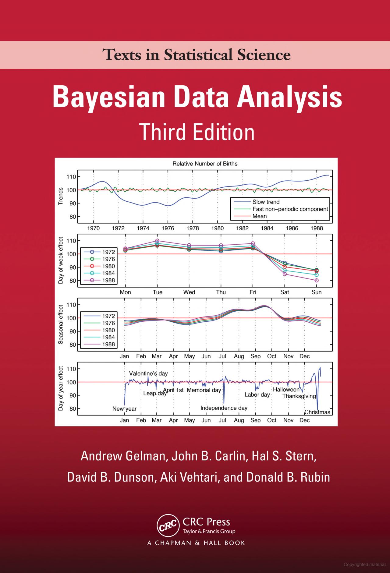
Bayesian Data Analysis
c.f. (Gelman et al. 2013)
- Title:Bayesian Data Analysis
- ISBN:1439840954, 9781439840955
- Page count:675
- Published:2013
- Format:Hardcover
- Publisher:Chapman and Hall/CRC
- Authors: Andrew Gelman, John B. Carlin, Hal S. Stern, David B. Dunson, Aki Vehtari, Donald B. Rubin
(Gelman et al. 2013) “Bayesian Data Analysis” is probably the most famous book on Bayesian statistics. This book is a classic text on Bayesian statistics and covers a wide range of topics in Bayesian data analysis. Although this is not a time series book, the authors have been intersted in the domain of political election prediction and have used time series data in their research and some of that is covered in the book’s examples.
- Audience: The book is suitable for graduate students and researchers in statistics, computer science, and related fields.
- An electronic version of the third eddition book is available at Bayesian Data Analysis
Introductory Time Series with R c.f. (Cowpertwait and Metcalfe 2009)
(Cowpertwait and Metcalfe 2009) “Introductory Time Series with R” by Cowpertwait and Metcalfe, and the second is
Yearly global mean temperature and ocean levels, daily share prices, and the signals transmitted back to Earth by the Voyager space craft are all examples of sequential observations over time known as time series. This book gives you a step-by-step introduction to analysing time series using the open source software R. Each time series model is motivated with practical applications, and is defined in mathematical notation. Once the model has been introduced it is used to generate synthetic data, using R code, and these generated data are then used to estimate its parameters. This sequence enhances understanding of both the time series model and the R function used to fit the model to data. Finally, the model is used to analyse observed data taken from a practical application. By using R, the whole procedure can be reproduced by the reader.
All the data sets used in the book are available on the website at datasets
The book is written for undergraduate students of mathematics, economics, business and finance, geography, engineering and related disciplines, and postgraduate students who may need to analyse time series as part of their taught programme or their research.
Paul Cowpertwait is an associate professor in mathematical sciences (analytics) at Auckland University of Technology with a substantial research record in both the theory and applications of time series and stochastic models.
Andrew Metcalfe is an associate professor in the School of Mathematical Sciences at the University of Adelaide, and an author of six statistics text books and numerous research papers. Both authors have extensive experience of teaching time series to students at all levels.
Analysis of Integrated and Cointegrated Time Series with R c.f.
(Pfaff 2008) “Analysis of Integrated and Cointegrated Time Series with R” by Bernhard Pfaff. Its been a long time since I read this book and rather than do it an injustice I direct you to the review by Dirk Eddelbuettel in the Journal of Statistical Software is avaoilable at review. Or the book’s website at Analysis of Integrated and Cointegrated Time Series with R.
The analysis of integrated and co-integrated time series can be considered as the main methodology employed in applied econometrics. This book not only introduces the reader to this topic but enables him to conduct the various unit root tests and co-integration methods on his own by utilizing the free statistical programming environment R. The book encompasses seasonal unit roots, fractional integration, coping with structural breaks, and multivariate time series models. The book is enriched by numerous programming examples to artificial and real data so that it is ideally suited as an accompanying text book to computer lab classes.
The second edition adds a discussion of vector auto-regressive, structural vector auto-regressive, and structural vector error-correction models.
Bayesian Analysis of Time Series by Lyle D. Broemeling
- covers pretty much the material in the course.
- uses winbugs and R
- models considered include
- white noise
- Wiener process (random walk)
- AR(p)
- ARMA(p,q)
- ARIMA
- Regression
- Regression with MA and Seasonal effects
- DLM
- TAR
Bayesian Inference for Stochastic Processes by Lyle D. Broemeling
- The code for R and WinBUGS is available at code
- IT is based on WinBUGS which is a bit dated but still useful.
- This books seems a bit dated but it covers a lot of the material in the course.
Dynamic Time Series Models using R-INLA: An Applied Perspective
(Ravishanker, Raman, and Soyer 2022) is a new book that covers the use of the R-INLA package for fitting dynamic time series models. The book is available online gitbook
This is a very interesting book which covers a new approach to fitting time series models using the R-INLA package. INLA stands for Integrated Nested Laplace Approximation and is a method for fitting Bayesian models that is faster than MCMC. The book covers a wide range of topics in time series modeling, computation, and inference. The book is suitable for graduate students and researchers in statistics, computer science, and related fields.
Statistics for Spatio-Temporal Data
(Cressie and Wikle 2011) is a book I came across when I tried to understand the NDLM model. NLDMs have a two level hierarcial form and it seems possible to extend this formulation will non-normaly distributed shocks and possibly non linear relation. In this book the authors take an interesting approch of not only looking at NDLM as a heirarchical model but they also extend the time series model into a spatio-temporal model.
This book is a comprehensive introduction to the analysis of spatio-temporal data and covers a wide range of topics in spatio-temporal statistics. The book is suitable for graduate students and researchers in statistics, computer science, and related fields.
Bayesian Analysis of Stochastic Process Models
c.f. (Rios Insua, Ruggeri, and Wiper 2012)
David Rios Insua, Fabrizio Ruggeri, Michael P. Wiper
This book is a comprehensive introduction to the analysis of stochastic process models using Bayesian methods. The book covers a wide range of topics in stochastic process modeling, computation, and inference. The book is suitable for graduate students and researchers in statistics, computer science, and related fields.
There are also a number of books on NDLM that I’ve come accross:
Forecasting, structural time series and the Kalman filter by Andrew C. Harvey
Dynamic Linear Models with R by Giovanni Petris Sonia Petrone Patrizia Campagnoli
Time Series Analysis by State Space Methods by J. Durbin and S.J. Koopman
References
Reuse
Citation
@online{bochman2024,
  author = {Bochman, Oren},
  title = {Week 0: {Introductions} to Time Series Analysis and the
    {AR(1)} Process},
  date = {2024-10-22},
  url = {https://orenbochman.github.io/notes/bayesian-ts/module0.html},
  langid = {en}
}
