Week 1: Introduction to Time Series and the AR(1) process

Learning Objectives

List the goals of the course
identify the basics of the R environment.
Explain stationary time series processes
Define auto-correlation function (ACF) and partial auto-correlation function (PACF) and use R to plot the sample ACF and sample PACF of a time series
Explain the concepts of differencing and smoothing via moving averages to remove/highlight trends and seasonal components in a time series
Define the zero-mean autoregressive process of order one or AR(1) and use R to obtain samples from this type of process
Perform maximum likelihood estimation for the full and conditional likelihood in an AR(1)
Perform Bayesian inference for the AR(1) under the conditional likelihood and the reference prior

Introduction

Welcome to Bayesian Statistics: Time Series

Obligatory introduction to the course and the instructors.
Raquel Prado is a professor of statistics in the Baskin School of Engineering at the University of California, Santa Cruz. She was the reciepient 2022 Zellner Medal, see Weckerle (2022)

Introduction to R

Introduction to R

The first two are the course textbooks.
The third is a classic text on machine learning which covers Durban-Levinson recursion and the Yule-Walker equations mentioned in the course.
The fourth is a classic text on statistical learning theory which covers the basics of time series analysis.

Stationarity the ACF and the PACF

Stationarity (video)

Stationarity is a key concept in time series analysis. A time series is said to be stationary if its statistical properties such as mean, variance, and auto-correlation do not change over time.

Notation

\{y_t\} - the time series process, where each y_t is a univariate random variable.
y_{1:T} or y_1, y_2, \ldots, y_T - the observed data.

Strong Stationarity: Strong Stationarity; given \{y_t\} for any n>0 and any h>0 and any subsequence the distribution of y_t, y_{t+1}, \ldots, y_{t+n} is the same as the distribution of y_{t+h}, y_{t+h+1}, \ldots, y_{t+h+n}.

since it is difficult to verify strong stationarity in practice, we often work with weak stationarity.

Weak Stationarity AKA Second-order Stationarity: Weak Stationarity; the mean, variance, and auto-covariance are constant over time.

strong stationarity implies weak stationarity, but
the converse is not true.
for a Gaussian process, our typical use case, they are equivalent!

Let y_t be a time series. We say that y_t is stationary if the following conditions hold:

The auto-correlation function ACF (video)

auto-correlation AFC

The partial auto-correlation function PACF (Reading)

Let {y_t} be a zero-mean stationary process.

Let

\hat{y}_t^{h-1} = \beta_1 y_{t-1} + \beta_2 y_{t-2} + \ldots + \beta_{h-1} y_{t-(h-1)}

be the best linear predictor of y_t based on the previous h − 1 values \{y_{t−1}, \ldots , y_{t−h+1}\}. The best linear predictor of y_t based on the previous h − 1 values of the process is the linear predictor that minimizes

E[(y_t − \hat{y}_y^{h-1})^2]

The partial autocorrelation of this process at lag h, denoted by \phi(h, h) is defined as:

partial auto-correlation PAFC

\phi(h, h) = Corr(y_{t+h} − \hat{y}_{t+h}^{h-1}, y_t − \hat{y}_t^{h-1})

for h ≥ 2 and \phi(1, 1) = Corr(y_{t+1}, y_{t}) = \rho(1).

The partial autocorrelation function can also be computed via the Durbin-Levinson recursion for stationary processes as \phi(0, 0) = 0,

\phi(n, n) = \frac{\rho(n) − \sum_{h=1}^{n-1} \phi(n − 1, h)\rho(n − h)}{1- \sum_{h=1}^{n-1}\phi(n − 1, h)\rho(h)}

for n ≥ 1, and

\phi(n, h) = \phi(n − 1, h) − \phi(n, n)\phi(n − 1, n − h),

for n ≥ 2, and h = 1, \ldots , (n − 1).

Note that the sample PACF can be obtained by substituting the sample autocorrelations and the sample auto-covariances in the Durbin-Levinson recursion.

Durbin-Levinson recursion (Off-Course Reading)

Like me, you might be curious about the Durbin-Levinson recursion mentioned above. This is not covered in the course, and turned out to be an enigma wrapped in a mystery.

I present my finding in the note below - much of it is due to (Wikipedia contributors 2024b) and (Wikipedia contributors 2024a)

In (Yule 1927) and (Walker 1931), Yule and Walker proposed a method for estimating the parameters of an autoregressive model. The method is based on the Yule-Walker equations which are a set of linear equations that can be used to estimate the parameters of an autoregressive model.

Due to the autoregressive nature of the model, the equations are take a special form called a Toeplitz matrix. However at the time they probably had to use the numerically unstable Gauss-Jordan elimination to solve these equations which is O(n^3) in time complexity.

A decade or two later in (Levinson 1946) and (Durbin 1960) the authors came up for with a weakly stable yet more efficient algorithm for solving these autocorrelated system of equations which requires only O(n^2) in time complexity. Later their work was further refined in (Trench 1964) and (Zohar 1969) to just 3\times n^2 multiplication. A cursory search reveals that Toeplitz matrix inversion is still an area of active research with papers covering parallel algorithms and stability studies. Not surprising as man of the more interesting deep learning models, including LLMs are autoregressive.

So the Durbin-Levinson recursion is just an elegant bit of linear algebra for solving the Yule-Walker equations more efficiently.

Here is what I dug up:

Durbin-Levinson and the Yule-Walker equations (Off-Course Reading)

The Durbin-Levinson recursion is a method in linear algebra for computing the solution to an equation involving a Toeplitz matrix AKA a diagonal-constant matrix where descending diagonals are constant. The recursion runs in O(n^2) time rather then O(n^3) time required by Gauss-Jordan elimination.

The recursion can be used to compute the coefficients of the autoregressive model of a stationary time series. It is based on the Yule-Walker equations and is used to compute the PACF of a time series.

The Yule-Walker equations can be stated as follows for an AR(p) process:

\gamma_m = \sum_{k=1}^p \phi_k \gamma_{m-k} + \sigma_\epsilon^2\delta_{m,0} \qquad \text{(Yule-Walker equations)} \tag{1}

where:

\gamma_m is the autocovariance function of the time series,
\phi_k are the AR coefficients,
\sigma_\epsilon^2 is the variance of the white noise process, and
\delta_{m,0} is the Kronecker delta function.

when m=0 the equation simplifies to:

\gamma_0 = \sum_{k=1}^p \phi_k \gamma_{-k} + \sigma_\epsilon^2 \qquad \text{(Yule-Walker equations for m=0)} \tag{2}

for m > 0 the equation simplifies to:

\begin{bmatrix} \gamma_1 \newline \gamma_2 \newline \gamma_3 \newline \vdots \newline \gamma_p \newline \end{bmatrix} = \begin{bmatrix} \gamma_0 & \gamma_{-1} & \gamma_{-2} & \cdots \newline \gamma_1 & \gamma_0 & \gamma_{-1} & \cdots \newline \gamma_2 & \gamma_1 & \gamma_0 & \cdots \newline \vdots & \vdots & \vdots & \ddots \newline \gamma_{p-1} & \gamma_{p-2} & \gamma_{p-3} & \cdots \newline \end{bmatrix} \begin{bmatrix} \phi_{1} \newline \phi_{2} \newline \phi_{3} \newline \vdots \newline \phi_{p} \newline \end{bmatrix}

and since this matrix is Toeplitz, we can use Durbin-Levinson recursion to efficiently solve the system for \phi_k \forall k.

Once \{\phi_m ; m=1,2, \dots ,p \} are known, we can consider m=0 and solved for \sigma_\epsilon^2 by substituting the \phi_k into Equation 2 Yule-Walker equations.

Of course the Durbin-Levinson recursion is not the last word on solving this system of equations. There are today numerous improvements which are both faster and more numerically stable.

Differencing and smoothing (Reading)

Many time series models are built under the assumption of stationarity. However, time series data often present non-stationary features such as trends or seasonality. Practitioners may consider techniques for detrending, deseasonalizing and smoothing that can be applied to the observed data to obtain a new time series that is consistent with the stationarity assumption.

We briefly discuss two methods that are commonly used in practice for detrending and smoothing.

Differencing

The first method is differencing, which is generally used to remove trends in time series data. The first difference of a time series is defined in terms of the so called difference operator denoted as D, that produces the transformation

differencing operator

Dy_t = y_t - y_{t-1}.

Higher order differences are obtained by successively applying the operator D. For example, D^2y_t = D(Dy_t) = D(y_t - y_{t-1}) = y_t - 2y_{t-1} + y_{t-2}.

Differencing can also be written in terms of the so called backshift operator B, with By_t = y_{t-1},

backshift operator

so that Dy_t = (1 - B)y_t and D^dy_t = (1 - B)d y_t.

Smoothing

The second method we discuss is moving averages, which is commonly used to “smooth” a time series by removing certain features (e.g., seasonality) to highlight other features (e.g., trends). A moving average is a weighted average of the time series around a particular time t. In general, if we have data y1:T , we could obtain a new time series such that

moving average

z_t = \sum_{j=-q}^{p} w_j y_{t+j},

for t = (q + 1) : (T − p), with weights w_j ≥ 0 and \sum^p_{j=−q} w_j = 1

We will frequently work with moving averages for which p = q \qquad \text{(centered)}

and

w_j = w_{−j} \forall j \text{(symmetric)}

Assume we have periodic data with period d. Then, symmetric and centered moving averages can be used to remove such periodicity as follows:

If d = 2q : z_t = \frac{1}{2} (y_{t−q} + y_{t−q+1} + \ldots + y_{t+q−1} + y_{t+q})
if d = 2q + 1 :

z_t = \frac{1}{d} (y_{t−q} + y_{t−q+1} + \ldots + y_{t+q−1} + y_{t+q})

Example: To remove seasonality in monthly data (i.e., seasonality with a period of d = 12 months), one can use a moving average with p = q = 6, a_6 = a_{−6} = 1/24, and a_j = a_{−j} = 1/12 for j = 0, \ldots , 5 , resulting in:

z_t = \frac{1}{12} (y_{t−6} + y_{t−5} + \ldots + y_{t+5} + y_{t+6})

ACF PACF Differencing and Smoothing Examples (Video)

Etiam non efficitur urna, quis elementum nisi. Mauris posuere a augue vel gravida. Praesent luctus erat et ex iaculis interdum. Nulla vestibulum quam ac nunc consequat vulputate. Nullam iaculis lobortis sem sit amet fringilla. Aliquam semper, metus ut blandit semper, nulla velit fermentum sapien, fermentum ultrices dolor sapien sed leo. Vestibulum molestie faucibus magna, at feugiat nulla ullamcorper a. Aliquam erat volutpat. Praesent scelerisque magna a justo maximus, sit amet suscipit mauris tempor. Nulla nec dolor eget ipsum pellentesque lobortis a in ipsum. Morbi turpis turpis, fringilla a eleifend maximus, viverra nec neque. Class aptent taciti sociosqu ad litora torquent per conubia nostra, per inceptos himenaeos.

Duis urna urna, pellentesque eu urna ut, malesuada bibendum dolor. Suspendisse potenti. Vivamus ornare, arcu quis molestie ultrices, magna est accumsan augue, auctor vulputate erat quam quis neque. Nullam scelerisque odio vel ultricies facilisis. Ut porta arcu non magna sagittis lacinia. Cras ornare vulputate lectus a tristique. Pellentesque ac arcu congue, rhoncus mi id, dignissim ligula.

R code for Differencing and filtering via moving averages (reading)

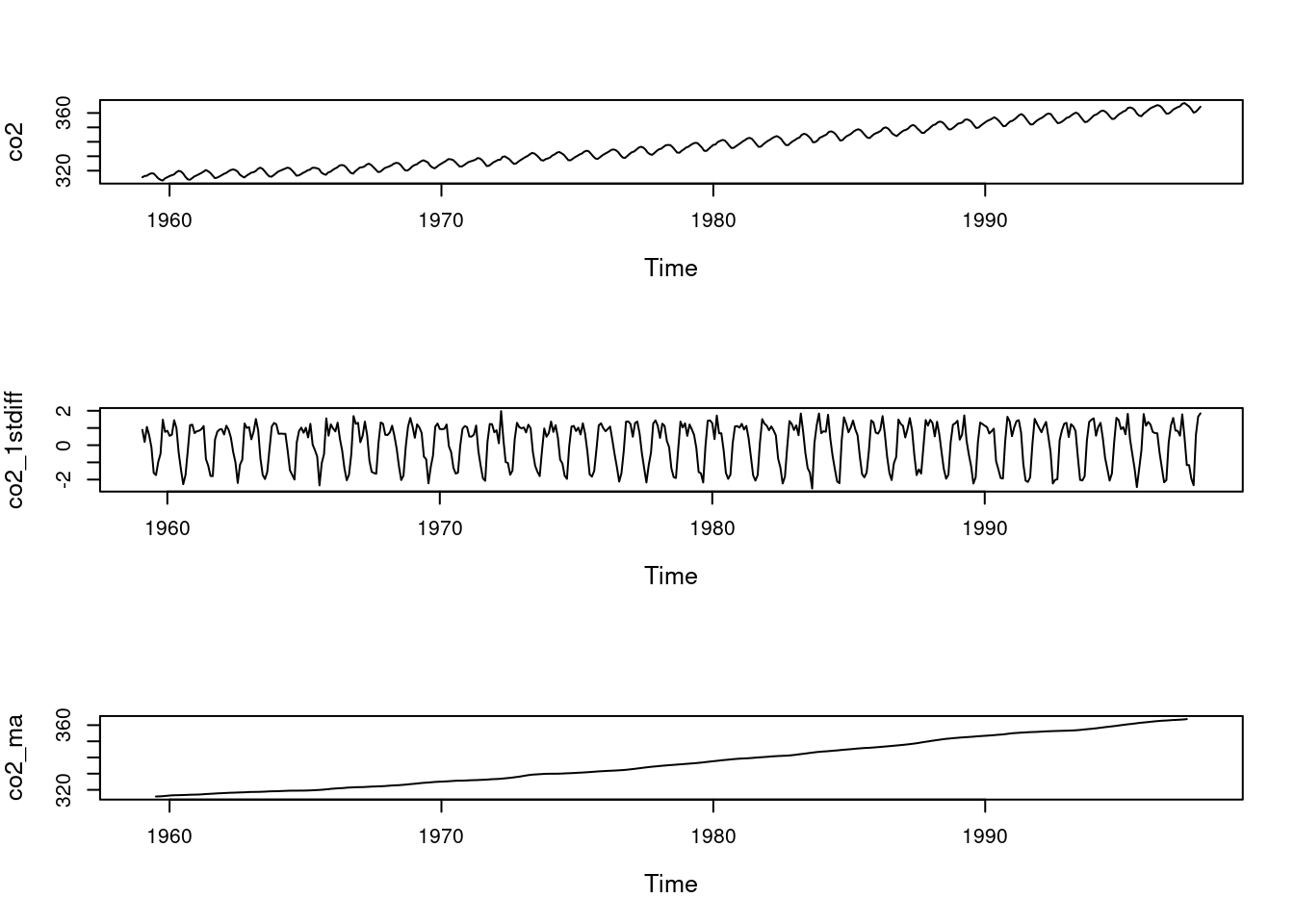
Code

# Load the CO2 dataset in R
data(co2) 

# Take first differences to remove the trend 
co2_1stdiff=diff(co2,differences=1)

# Filter via moving averages to remove the seasonality 
co2_ma=filter(co2,filter=c(1/24,rep(1/12,11),1/24),sides=2)

par(mfrow=c(3,1), cex.lab=1.2,cex.main=1.2)
plot(co2) # plot the original data 
plot(co2_1stdiff) # plot the first differences (removes trend, highlights seasonality)
plot(co2_ma) # plot the filtered series via moving averages (removes the seasonality, highlights the trend)

R Code: Simulate data from a white noise process

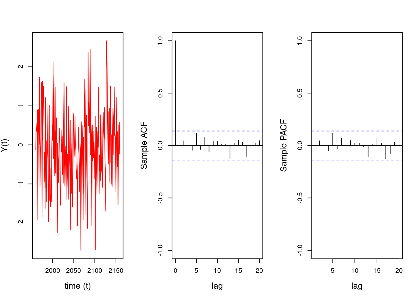
Code

#
# Simulate data with no temporal structure (white noise)
#
set.seed(2021)
T=200
t =1:T
y_white_noise=rnorm(T, mean=0, sd=1)
#
# Define a time series object in R: 
# Assume the data correspond to annual observations starting in January 1960 
#
yt=ts(y_white_noise, start=c(1960), frequency=1)
#
# plot the simulated time series, their sample ACF and their sample PACF
#
par(mfrow = c(1, 3), cex.lab = 1.3, cex.main = 1.3)
yt=ts(y_white_noise, start=c(1960), frequency=1)
plot(yt, type = 'l', col='red', xlab = 'time (t)', ylab = "Y(t)")
acf(yt, lag.max = 20, xlab = "lag",
    ylab = "Sample ACF",ylim=c(-1,1),main="")
pacf(yt, lag.max = 20,xlab = "lag",
     ylab = "Sample PACF",ylim=c(-1,1),main="")

Quiz 1: Stationarity, ACF, PACF, Differencing, and Smoothing

omitted per corsera requirements

The AR(1) process: Definition and properties

Aenean placerat luctus tortor vitae molestie. Nulla at aliquet nulla. Sed efficitur tellus orci, sed fringilla lectus laoreet eget. Vivamus maximus quam sit amet arcu dignissim, sed accumsan massa ullamcorper. Sed iaculis tincidunt feugiat. Nulla in est at nunc ultricies dictum ut vitae nunc. Aenean convallis vel diam at malesuada. Suspendisse arcu libero, vehicula tempus ultrices a, placerat sit amet tortor. Sed dictum id nulla commodo mattis. Aliquam mollis, nunc eu tristique faucibus, purus lacus tincidunt nulla, ac pretium lorem nunc ut enim. Curabitur eget mattis nisl, vitae sodales augue. Nam felis massa, bibendum sit amet nulla vel, vulputate rutrum lacus. Aenean convallis odio pharetra nulla mattis consequat.

Ut ut condimentum augue, nec eleifend nisl. Sed facilisis egestas odio ac pretium. Pellentesque consequat magna sed venenatis sagittis. Vivamus feugiat lobortis magna vitae accumsan. Pellentesque euismod malesuada hendrerit. Ut non mauris non arcu condimentum sodales vitae vitae dolor. Nullam dapibus, velit eget lacinia rutrum, ipsum justo malesuada odio, et lobortis sapien magna vel lacus. Nulla purus neque, hendrerit non malesuada eget, mattis vel erat. Suspendisse potenti.

The AR(1) process (video)

Etiam congue quam eget velit convallis, eu sagittis orci vestibulum. Vestibulum at massa turpis. Curabitur ornare ex sed purus vulputate, vitae porta augue rhoncus. Phasellus auctor suscipit purus, vel ultricies nunc. Nunc eleifend nulla ac purus volutpat, id fringilla felis aliquet. Duis vitae porttitor nibh, in rhoncus risus. Vestibulum a est vitae est tristique vehicula. Proin mollis justo id est tempus hendrerit. Praesent suscipit placerat congue. Aliquam eu elit gravida, consequat augue non, ultricies sapien. Nunc ultricies viverra ante, sit amet vehicula ante volutpat id. Etiam tempus purus vitae tellus mollis viverra. Donec at ornare mauris. Aliquam sodales hendrerit ornare. Suspendisse accumsan lacinia sapien, sit amet imperdiet dui molestie ut.

The PACF of the AR(1) process (reading)

It is possible to show that the PACF of an autoregressive process of order one is zero after the first lag. We can use the Durbin-Levinson recursion to show this.

For lag n = 0 we have \phi(0, 0) = 0.

For lag n = 1 we have: \phi(1, 1) = \rho(1) = \phi

For lag n = 2 we compute \phi(2, 2) as:

\phi(2, 2) = \frac{(\rho(2) − \phi(1, 1)\rho(1))}{ (1 − \phi(1, 1)\rho(1))} = \frac{\phi^2-\phi^2}{1- \phi^2}=0

and we also obtain

\phi(2, 1) = \phi(1, 1) − \phi(2, 2)\phi(1, 1) = \phi.

For lag n = 3 we compute \phi(3, 3) as

\begin{align*} \phi(3, 3) &= \frac{(\rho(3) − \sum_{h=1}^2 \phi(2, h)\rho(3 − h))}{1 − \sum_{h=1}^2 \phi(2, h)\rho(h)} \newline &= \frac{\phi^3 - \phi(2,1) \rho(2) - \phi(2,2) \rho(1)}{1 - \phi(2,1)\rho(1) - \phi(2,2)\rho(2)} \newline &= \frac{\phi^3 - \phi^3 - 0}{1 - \phi^2 } \newline &= 0 \end{align*}

and we also obtain

\phi(3, 1) = \phi(2, 1) − \phi(3, 3)\phi(2, 2) = \phi

\phi(3, 2) = \phi(2, 2) − \phi(3, 3)\phi(2, 1) = 0

We can prove by induction that in the case of an AR(1), for any lag n,

\phi(n, h) = 0, \phi(n, 1) = \phi and \phi(n, h) = 0 for h ≥ 2 and n ≥ 2.

Then, the PACF of an AR(1) is zero for any lag above 1 and the PACF coefficient at lag 1 is equal to the AR coefficient \phi

Etiam maximus accumsan gravida. Maecenas at nunc dignissim, euismod enim ac, bibendum ipsum. Maecenas vehicula velit in nisl aliquet ultricies. Nam eget massa interdum, maximus arcu vel, pretium erat. Maecenas sit amet tempor purus, vitae aliquet nunc. Vivamus cursus urna velit, eleifend dictum magna laoreet ut. Duis eu erat mollis, blandit magna id, tincidunt ipsum. Integer massa nibh, commodo eu ex vel, venenatis efficitur ligula. Integer convallis lacus elit, maximus eleifend lacus ornare ac. Vestibulum scelerisque viverra urna id lacinia. Vestibulum ante ipsum primis in faucibus orci luctus et ultrices posuere cubilia curae; Aenean eget enim at diam bibendum tincidunt eu non purus. Nullam id magna ultrices, sodales metus viverra, tempus turpis.

Duis ornare ex ac iaculis pretium. Maecenas sagittis odio id erat pharetra, sit amet consectetur quam sollicitudin. Vivamus pharetra quam purus, nec sagittis risus pretium at. Nullam feugiat, turpis ac accumsan interdum, sem tellus blandit neque, id vulputate diam quam semper nisl. Donec sit amet enim at neque porttitor aliquet. Phasellus facilisis nulla eget placerat eleifend. Vestibulum non egestas eros, eget lobortis ipsum. Nulla rutrum massa eget enim aliquam, id porttitor erat luctus. Nunc sagittis quis eros eu sagittis. Pellentesque dictum, erat at pellentesque sollicitudin, justo augue pulvinar metus, quis rutrum est mi nec felis. Vestibulum efficitur mi lorem, at elementum purus tincidunt a. Aliquam finibus enim magna, vitae pellentesque erat faucibus at. Nulla mauris tellus, imperdiet id lobortis et, dignissim condimentum ipsum. Morbi nulla orci, varius at aliquet sed, facilisis id tortor. Donec ut urna nisi.

Sample data from AR(1) processes (Reading)

Code

# sample data from 2 ar(1) processes and plot their ACF and PACF functions
#
set.seed(2021)
T=500 # number of time points
#
# sample data from an ar(1) with ar coefficient phi = 0.9 and variance 1
#
v=1.0 # innovation variance
sd=sqrt(v) #innovation stantard deviation
phi1=0.9 # ar coefficient
yt1=arima.sim(n = T, model = list(ar = phi1), sd = sd)
#
# sample data from an ar(1) with ar coefficient phi = -0.9 and variance 1
#
phi2=-0.9 # ar coefficient
yt2=arima.sim(n = T, model = list(ar = phi2), sd = sd)

par(mfrow = c(2, 1), cex.lab = 1.3)
plot(yt1,main=expression(phi==0.9))
plot(yt2,main=expression(phi==-0.9))

Code

par(mfrow = c(3, 2), cex.lab = 1.3)
lag.max=50 # max lag
#
## plot true ACFs for both processes
#
cov_0=sd^2/(1-phi1^2) # compute auto-covariance at h=0
cov_h=phi1^(0:lag.max)*cov_0 # compute auto-covariance at h
plot(0:lag.max, cov_h/cov_0, pch = 1, type = 'h', col = 'red',
     ylab = "true ACF", xlab = "Lag",ylim=c(-1,1), main=expression(phi==0.9))

cov_0=sd^2/(1-phi2^2) # compute auto-covariance at h=0
cov_h=phi2^(0:lag.max)*cov_0 # compute auto-covariance at h
# Plot autocorrelation function (ACF)
plot(0:lag.max, cov_h/cov_0, pch = 1, type = 'h', col = 'red',
     ylab = "true ACF", xlab = "Lag",ylim=c(-1,1),main=expression(phi==-0.9))

## plot sample ACFs for both processes
#
acf(yt1, lag.max = lag.max, type = "correlation", ylab = "sample ACF",
    lty = 1, ylim = c(-1, 1), main = " ")
acf(yt2, lag.max = lag.max, type = "correlation", ylab = "sample ACF",
    lty = 1, ylim = c(-1, 1), main = " ")
## plot sample PACFs for both processes
#
pacf(yt1, lag.ma = lag.max, ylab = "sample PACF", ylim=c(-1,1),main="")
pacf(yt2, lag.ma = lag.max, ylab = "sample PACF", ylim=c(-1,1),main="")

Quiz 2: The AR(1) definition and properties

Omitted per Coursera requirements

The AR(1) process:Maximum likelihood estimation and Bayesian inference

References

Durbin, J. 1960. “The Fitting of Time-Series Models.” Revue de l’Institut International de Statistique / Review of the International Statistical Institute 28 (3): 233–44. http://www.jstor.org/stable/1401322.

Levinson, Norman. 1946. “The Wiener (Root Mean Square) Error Criterion in Filter Design and Prediction.” Journal of Mathematics and Physics 25 (1-4): 261–78. https://doi.org/https://doi.org/10.1002/sapm1946251261.

Prado, R., M. A. R. Ferreira, and M. West. 2023. Time Series: Modeling, Computation, and Inference. Chapman & Hall/CRC Texts in Statistical Science. CRC Press. https://books.google.co.il/books?id=pZ6lzgEACAAJ.

Storch, H. von, and F. W. Zwiers. 2002. Statistical Analysis in Climate Research. Cambridge University Press. https://books.google.co.il/books?id=bs8hAwAAQBAJ.

Theodoridis, S. 2015. Machine Learning: A Bayesian and Optimization Perspective. Elsevier Science. https://books.google.co.il/books?id=hxQRogEACAAJ.

Trench, William F. 1964. “An Algorithm for the Inversion of Finite Toeplitz Matrices.” Journal of the Society for Industrial and Applied Mathematics 12 (3): 515–22. http://ramanujan.math.trinity.edu/wtrench/research/papers/TRENCH_RP_6.PDF.

Walker, Gilbert Thomas. 1931. “On Periodicity in Series of Related Terms.” Proceedings of the Royal Society of London. Series A, Containing Papers of a Mathematical and Physical Character 131 (818): 518–32. https://doi.org/10.1098/rspa.1931.0069.

Weckerle, Melissa. 2022. “Statistics professor wins prestigious professional statistics society award Baskin School of Engineering.” https://engineering.ucsc.edu/news/statistics-professor-wins-zellner-medal.

West, M., and J. Harrison. 2013. Bayesian Forecasting and Dynamic Models. Springer Series in Statistics. Springer New York. https://books.google.co.il/books?id=NmfaBwAAQBAJ.

Wikipedia contributors. 2024a. “Autoregressive Model — Wikipedia, the Free Encyclopedia.” https://en.wikipedia.org/w/index.php?title=Autoregressive_model&oldid=1233171855#Estimation_of_AR_parameters.

———. 2024b. “Levinson Recursion — Wikipedia, the Free Encyclopedia.” https://en.wikipedia.org/w/index.php?title=Levinson_recursion&oldid=1229942891.

Yule, George Udny. 1927. “VII. On a Method of Investigating Periodicities Disturbed Series, with Special Reference to Wolfer’s Sunspot Numbers.” Philosophical Transactions of the Royal Society of London. Series A, Containing Papers of a Mathematical or Physical Character 226 (636-646): 267–98. https://doi.org/10.1098/rsta.1927.0007.

Zohar, Shalhav. 1969. “Toeplitz Matrix Inversion: The Algorithm of w. F. Trench.” J. ACM 16: 592–601. https://api.semanticscholar.org/CorpusID:3115290.

Reuse

CC SA BY-NC-ND

Citation

BibTeX citation:

@online{bochman2024,
  author = {Bochman, Oren},
  title = {Mixture {Models}},
  date = {2024-10-23},
  url = {https://orenbochman.github.io/notes/bayesian-mixtures/module1.html},
  langid = {en}
}

For attribution, please cite this work as:

Bochman, Oren. 2024. “Mixture Models.” October 23, 2024. https://orenbochman.github.io/notes/bayesian-mixtures/module1.html.