Machine learning models can be analyzed at a high level using global explanations, such as linear model coefficients. However, there are several limitations to these global explanations. In this talk, I will review the use cases where local explanations are needed and introduce two popular methods for generating local explanations LIME and SHAP. Our learning will be focused on SHAP, its theory, model-agnostic and model-specific versions, and how to use and read SHAP visualizations.
explainable AI
XAI
machine learning
ML
data science
contrafactuals
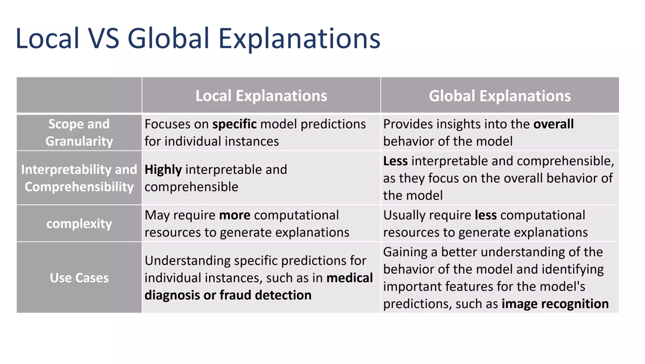
global explanations
local explanations
LIME
SHAP
CI
Author
Oren Bochman
Published
Monday, March 13, 2023
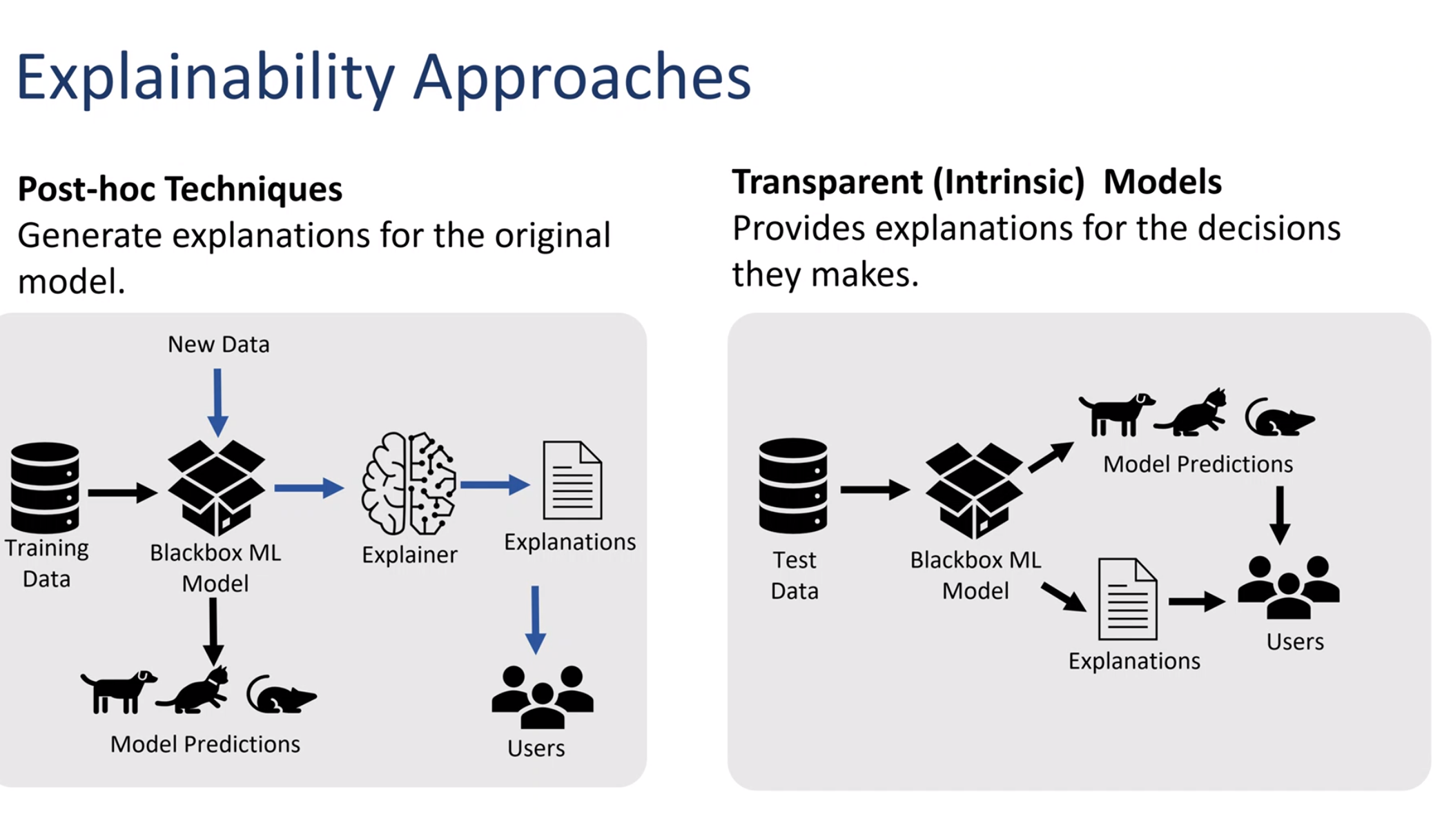
XAI is all about illuminating the opaque inner working of black box model. These are the type of models data scientist prefer to deploy to production as they tend to give better results. The rub is that many end users and other stakeholders like executives may not trust the predictions made by such models. After all we all learned that:
all model are wrong but some are useful.
XAI empowers the data scientist with post hoc methods that manipulate the black box model and make the outcomes more approachable to users.
There are added benefits - when we use local explanations to understand why the model is giving bad predictions for specific entries. This understanding is the best way to move forward and improve the model. We can also use these to understand the biases that tend to creep into our model so we can take steps to mitigate it.
This is a fascinating session on XAI, building on the previous session. I’ve embedded the video below.
The speakers did not provide code samples. I have tried to add some code samples but any shortcoming are mine.
Series Poster
series poster
Session Video
This is the video for this session:
Instructor Biographies
Bitya Neuhof
Ph.D student, Statistics & Data Science
HUJI
Bitya is a Ph.D. student in Statistics and Data Science at the Hebrew University, exploring and developing explainable AI methods. Before her PhD she worked as a Data Scientist specializing in analyzing high-dimensional tabular data. Bitya is also a Core-Team member at Baot, the largest Israeli community of experienced women in R&D.
Yasmin is a ML Scientist Leader and Mentor in the Startups Accelerator program at Microsoft. Her work focuses on developing (ML) models for Microsoft Cloud Computing Platforms and Services. Part of her work has been filed as patents, published in Microsoft Journal of Applied Research (MSJAR), and presented at various conferences, meetups and webinars. Previously her work focused on the security field developing ML models to detect cyber-attacks and methods to harvest leaked information in social networks using socialbots and crawler and detecting the source of the leak. She is listed as a cyber threat detection method patent author and part of her research was published at the IEEE/ACM International Conference on Advances in Social Networks Analysis and Mining. Yasmin graduated fast track for an MSc degree, that focused on ML & Security, in the department of Information Systems Engineering at Ben-Gurion University in Israel.
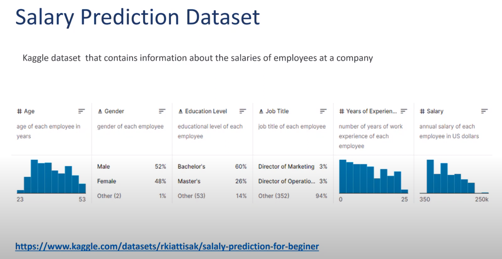
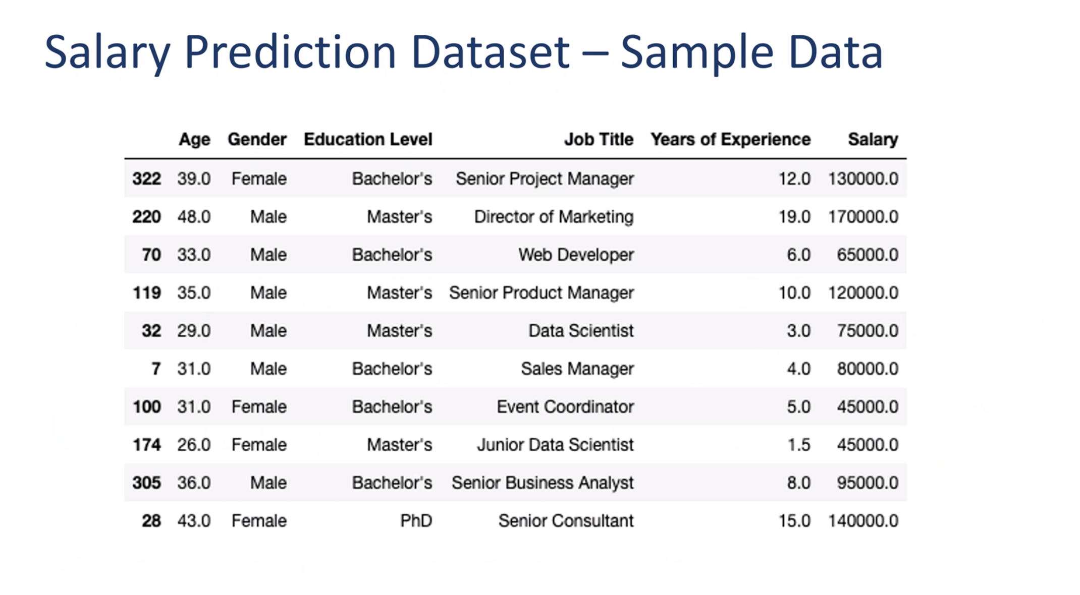
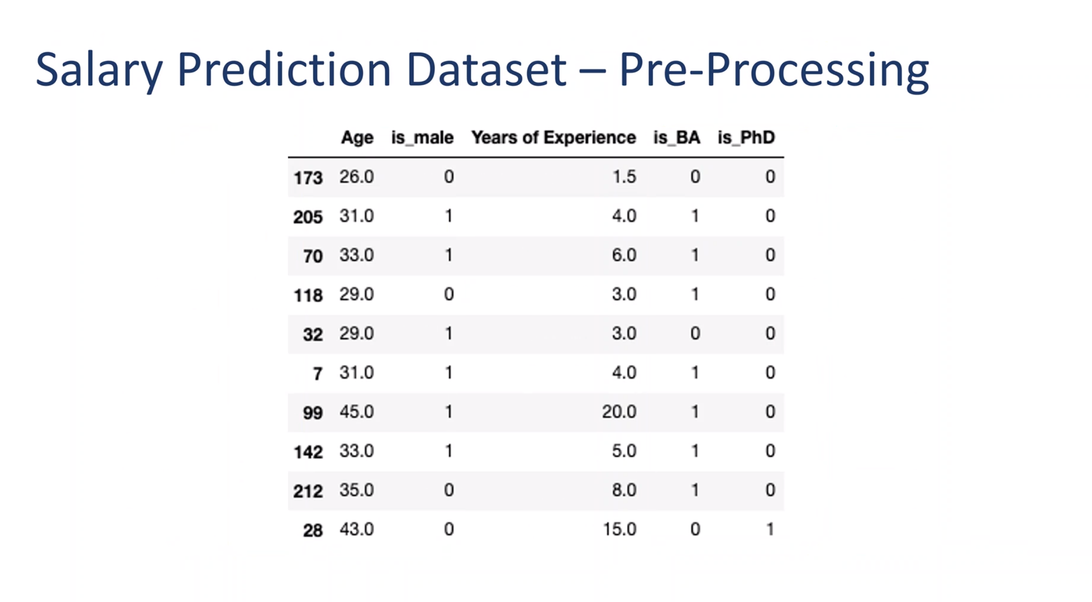
import numpy as npimport pandas as pdfrom itables import showimport matplotlib.pyplot as pltimport seaborn as snsfrom sklearn.model_selection import train_test_splitimport xgboost as xgbdf = pd.read_csv('./data/Salary Data.csv')show(df.head())
dt_clf_model = DecisionTreeRegressor( max_depth=3, random_state=123)dt_clf_model.fit(X_train, y_train)#Predict the response for test datasety_pred = dt_clf_model.predict(X_test)# Model Accuracy, how often is the classifier correct?#print("Accuracy:",metrics.accuracy_score(y_test, y_pred))
In a Jupyter environment, please rerun this cell to show the HTML representation or trust the notebook. On GitHub, the HTML representation is unable to render, please try loading this page with nbviewer.org.
/home/oren/work/blog/env/lib/python3.10/site-packages/sklearn/base.py:493: UserWarning:

X does not have valid feature names, but DecisionTreeRegressor was fitted with feature names
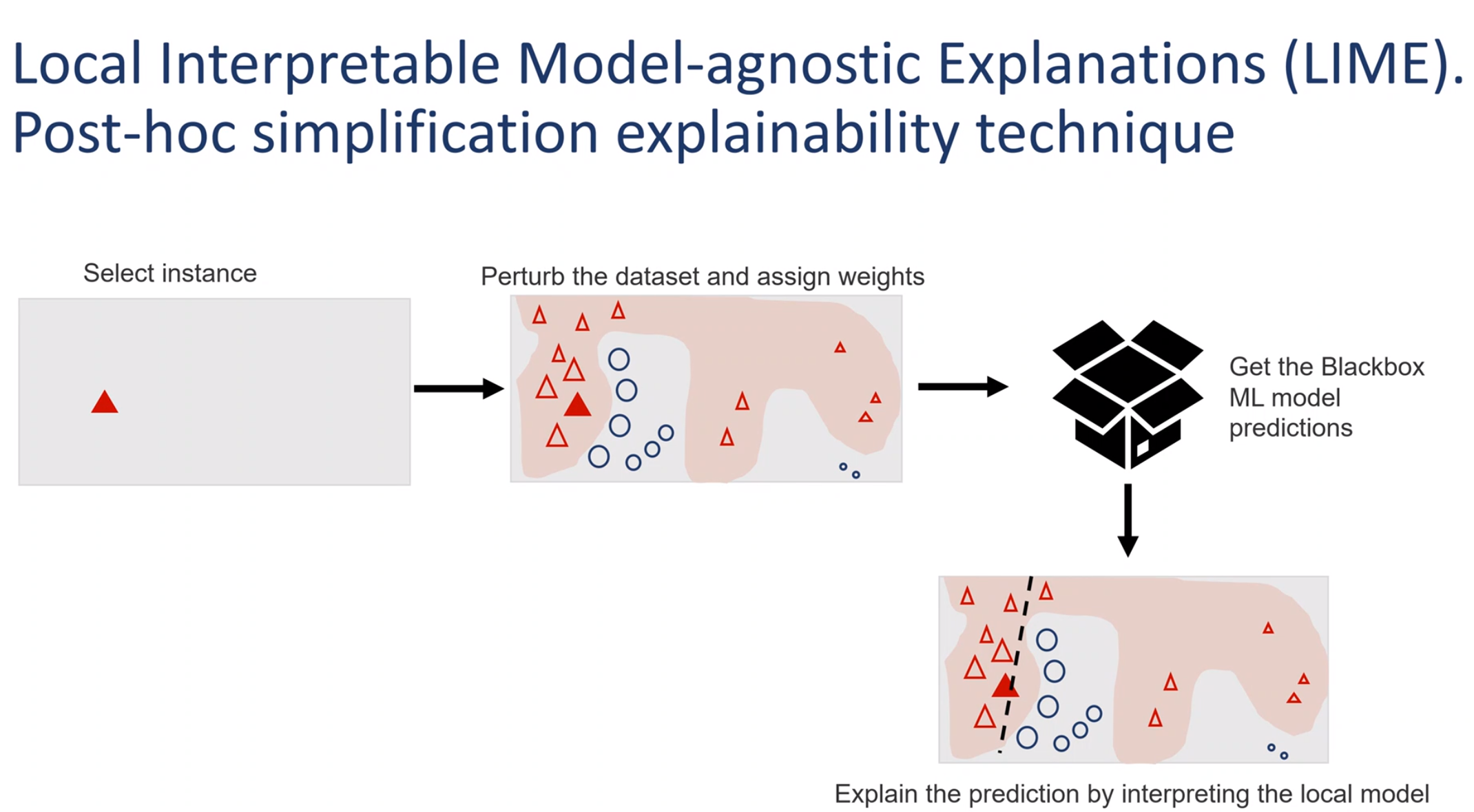
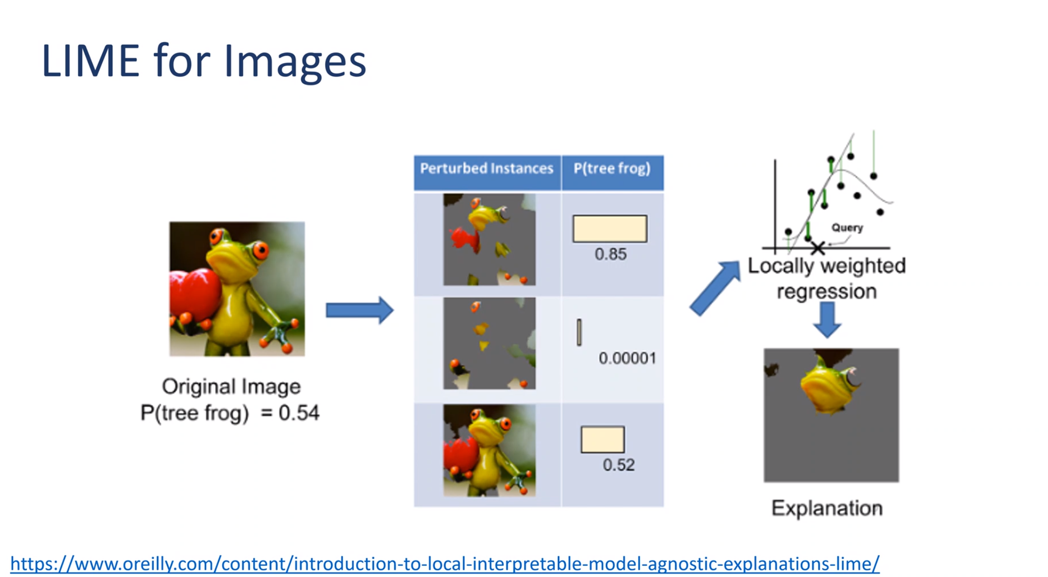
Our data is a complex manifold with non-convex boundry pink region
repeat:
We pick a single row r_i in the data set which we call an instance.
We then perturb it by modifying the instance randomly p_i=x_i + \delta
We generate a prediction for the perturbation using our black box model \hat y_{p_i}
We reweigh each perturbation using the relative distance of the prediction: w \propto | \hat{y} - \hat y_{p_i} |
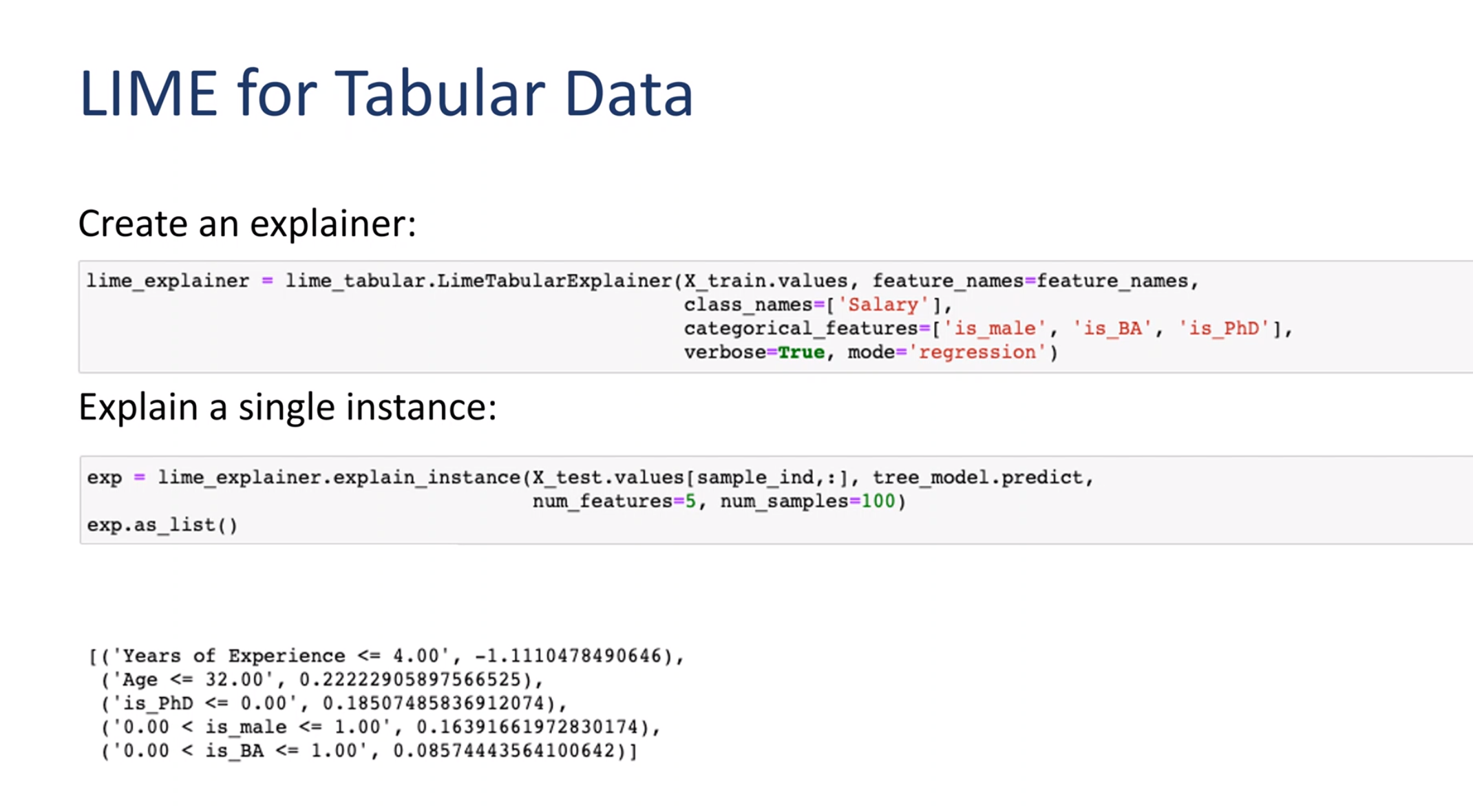
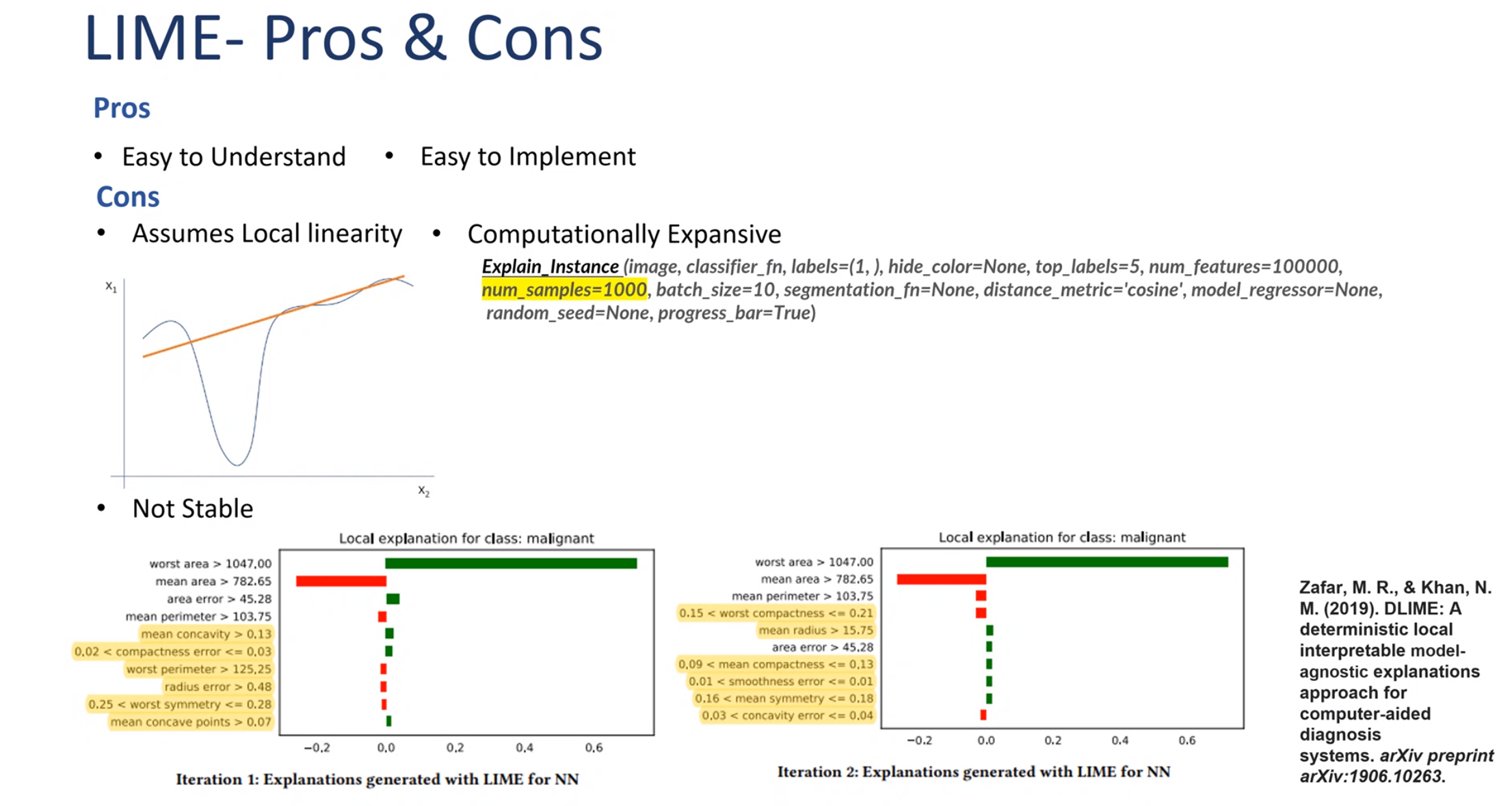
More precisely, the explanation for a data point x is the model g that minimizes the locality-aware loss L(f,g,Π_x) measuring how unfaithful g approximates the model to be explained f in its vicinity Π_x while keeping the model complexity denoted low.
\arg\min _g L(f,g,\pi_x)+\Omega(g)
Therefore, LIME experiences a trade off between model fidelity and complexity
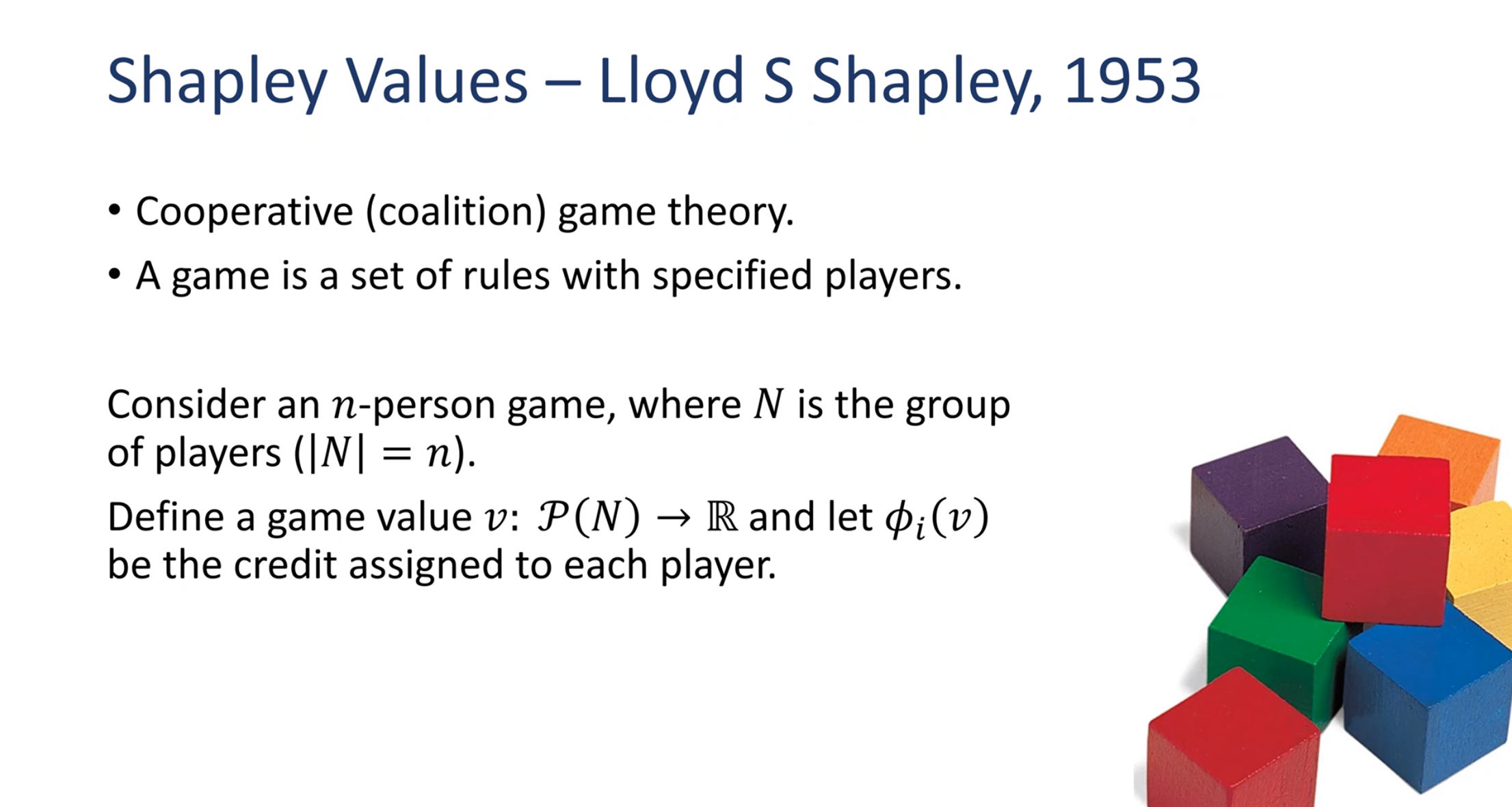
Far a cooperative game it considers all coalitions and lets us see how much each is contributing to overall surplus.
This idea can then be used to decide how divide the surplus (profit) most fairly.
Think how the extremest can set the tone for a coalition by threatening to break it up.
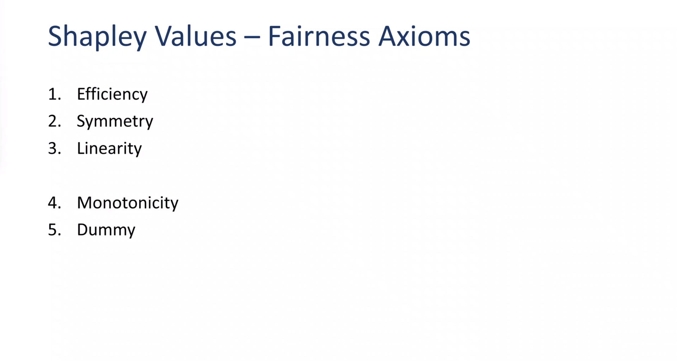
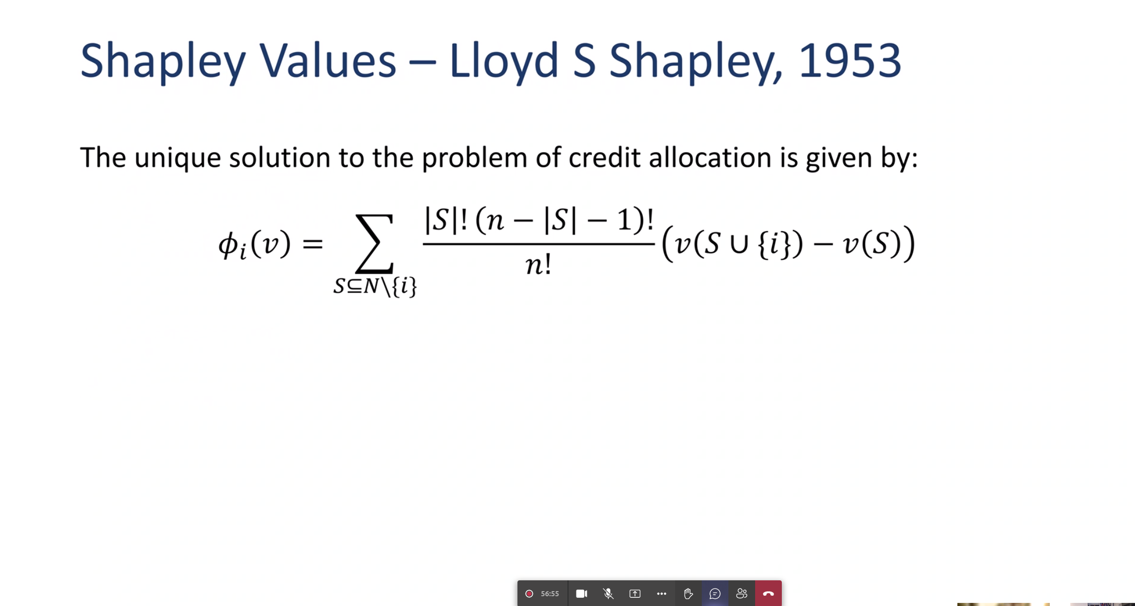
1. Efficiency - The sum of the Shapley values of all agents equals the value of the grand coalition, so that all the gain is distributed among the agents: 2. Symmetry - equal treatment of equals 3. Linearity - If two coalition games described by gain functions {\displaystyle v} and {\displaystyle w} are combined, then the distributed gains should correspond to the gains derived from {\displaystyle v} and the gains derived from {\displaystyle w} 4. Monotonically 5. Null Player - The Shapley value \varphi _{i}(v) of a null player i in a game v is zero.
Shapley Formula
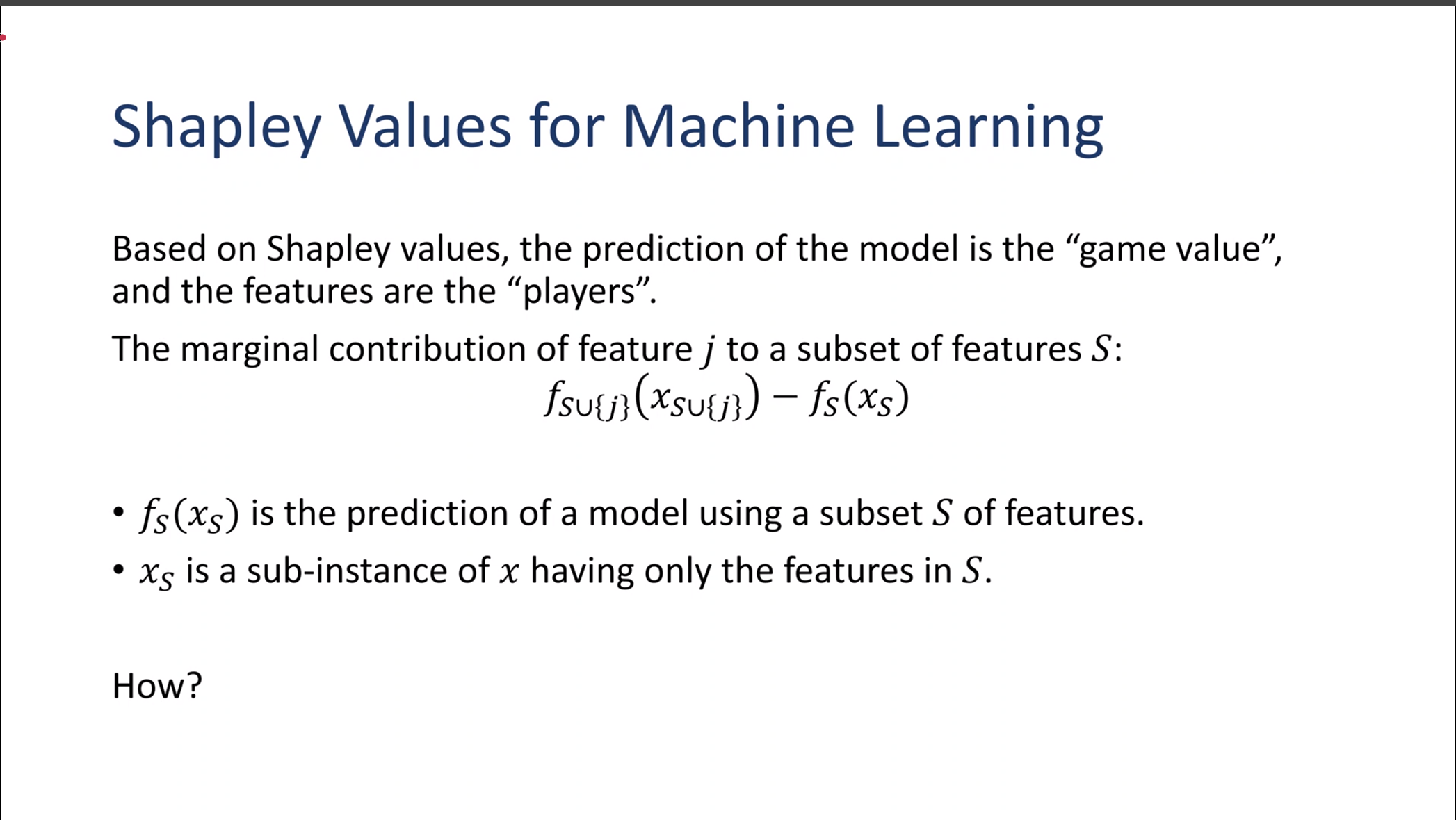
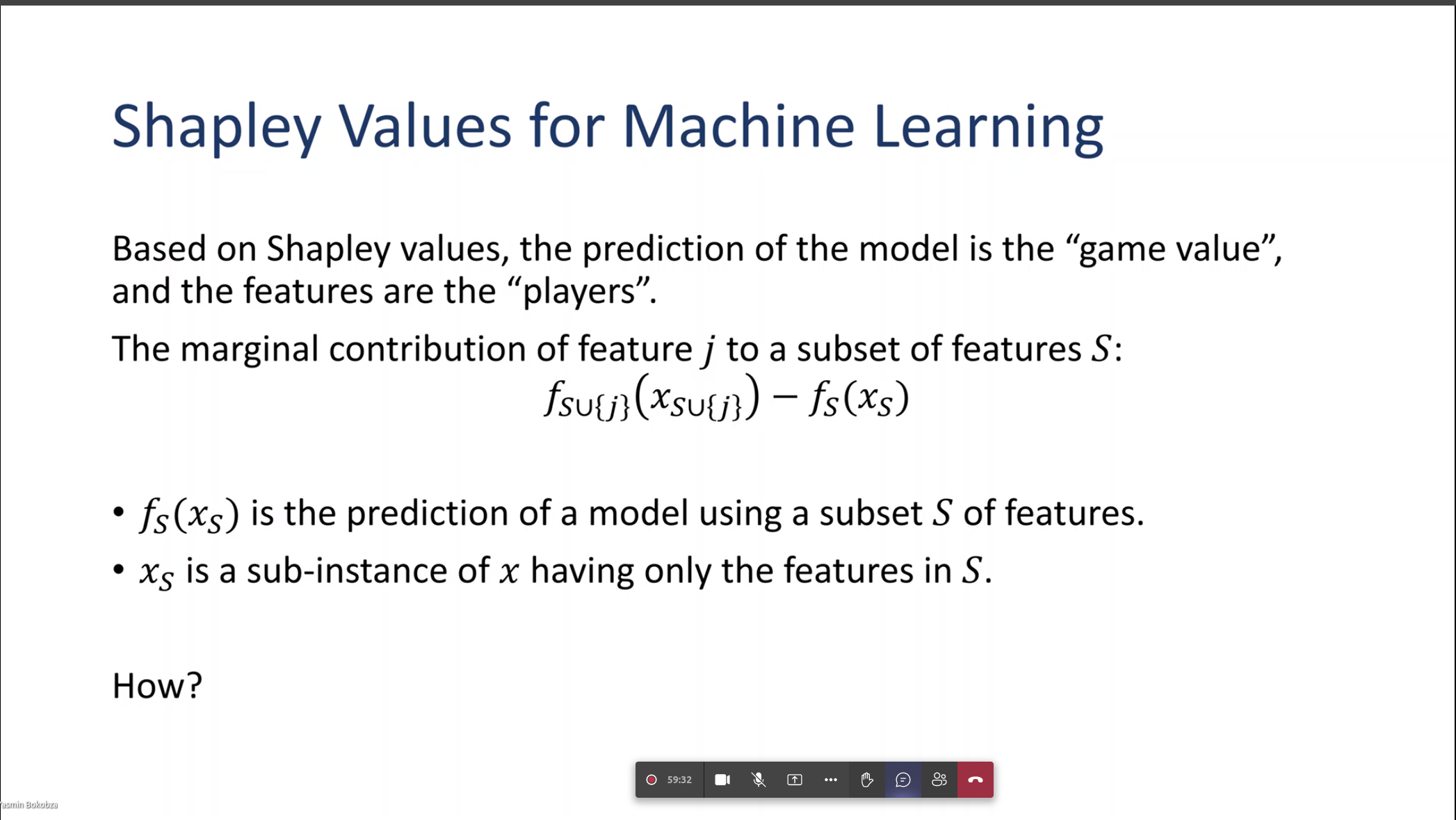
In ML
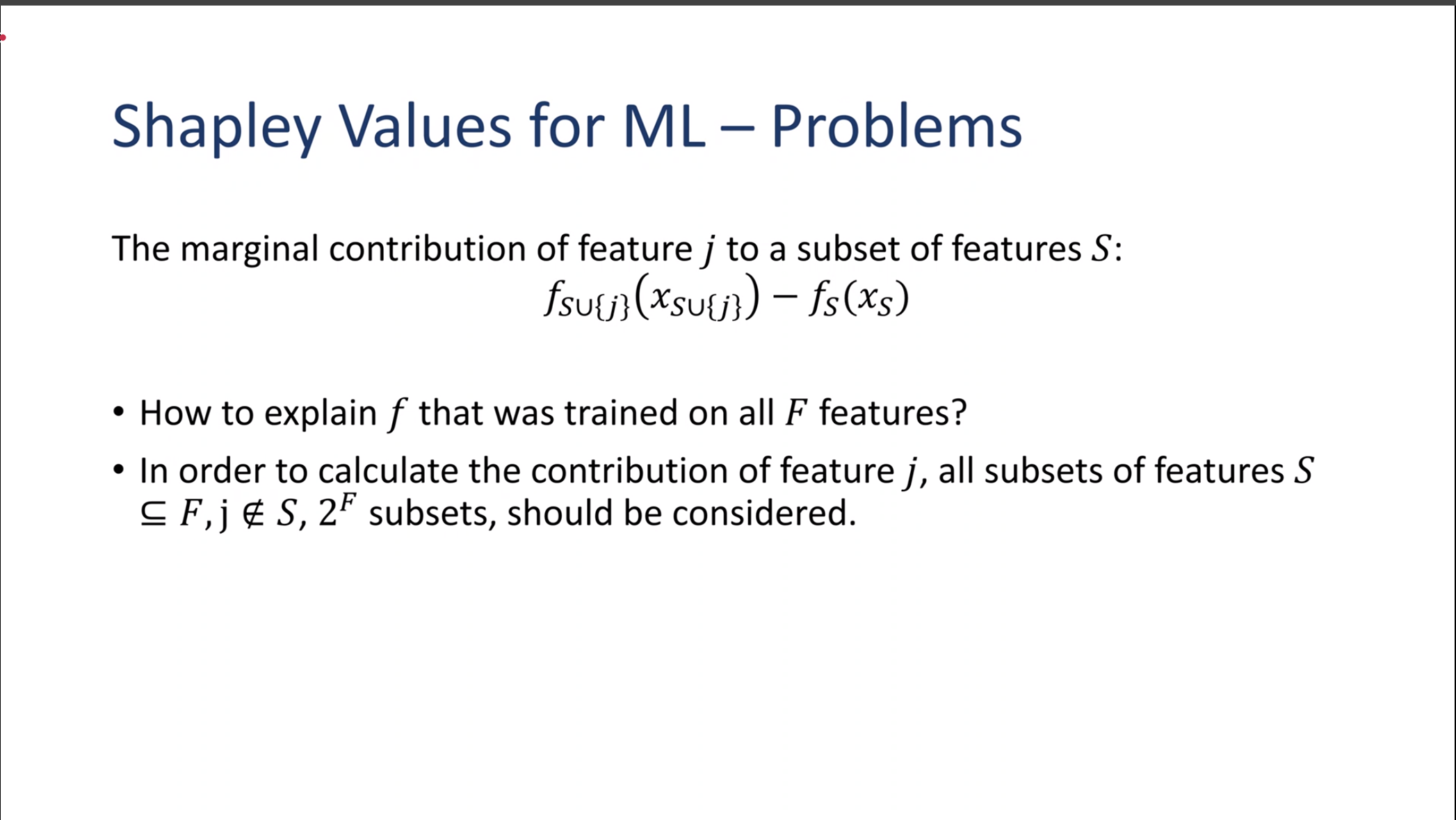
Shapley Problems
Shapley for ML
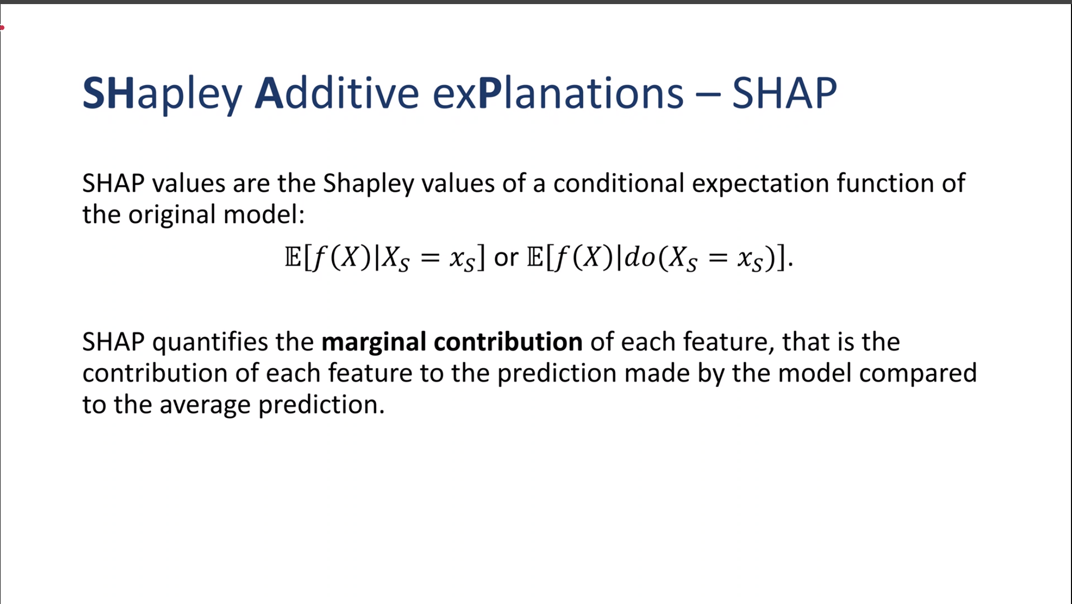
SHAP
SHAP - Shapley Addative Explanations
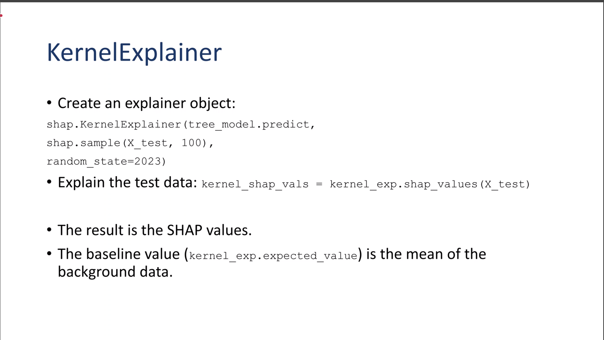
Kernel SHAP
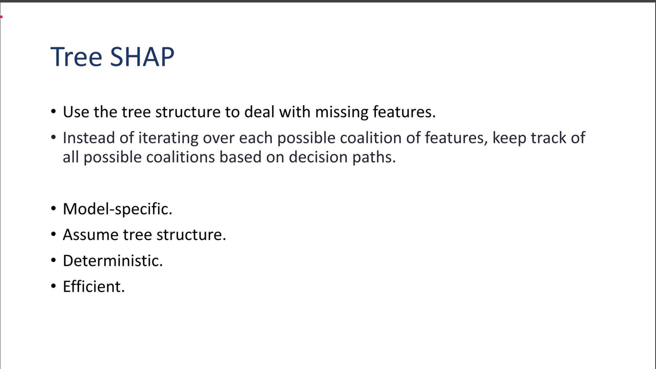
Tree SHAP
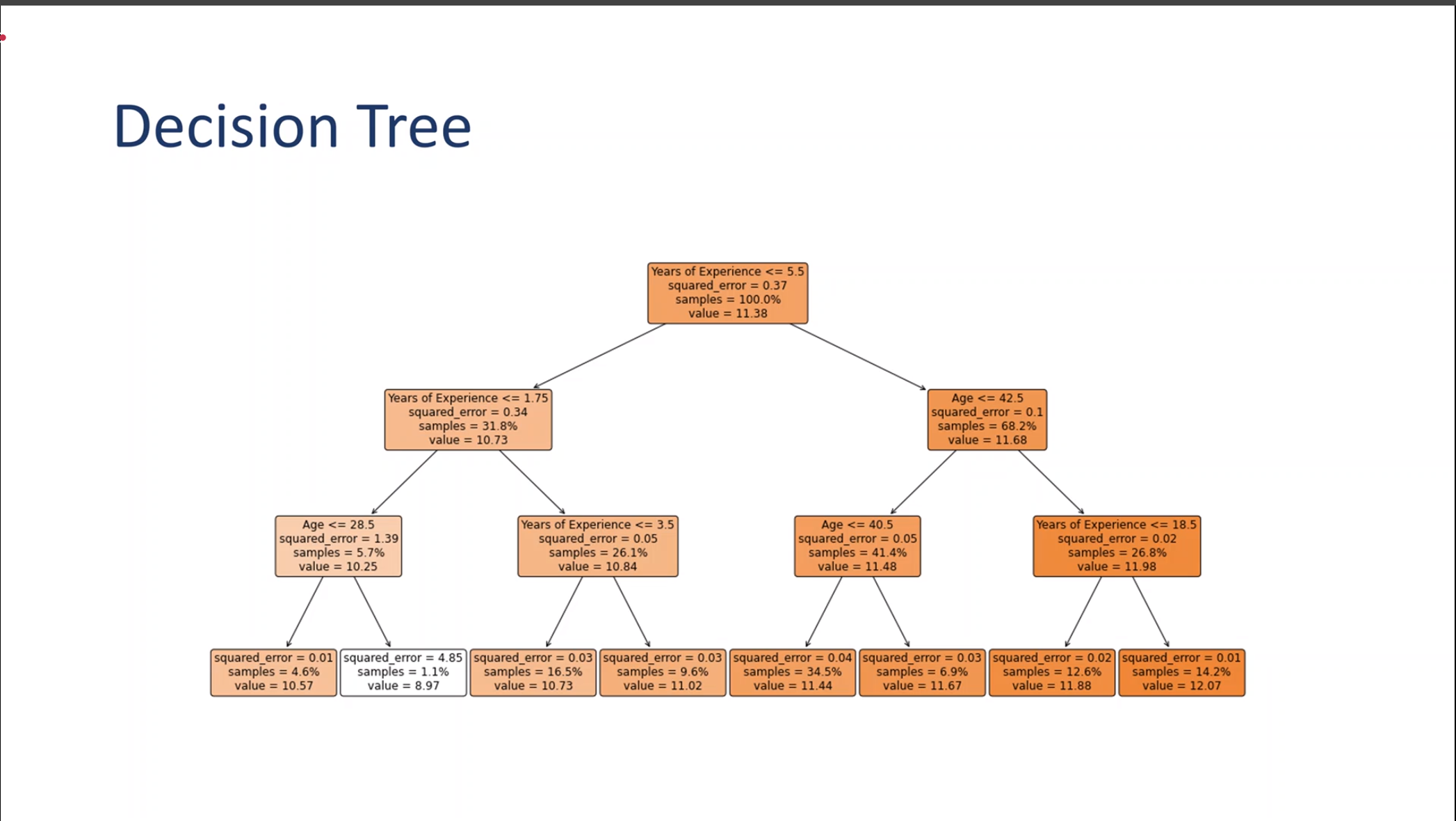
Decision Tree
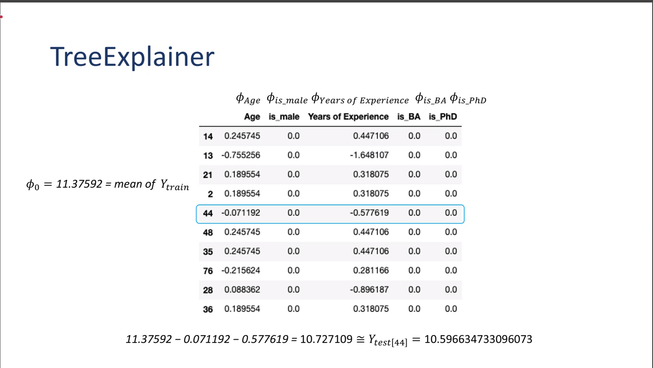
TreeExplainer
Kernel Explainer
SHAP Visualization
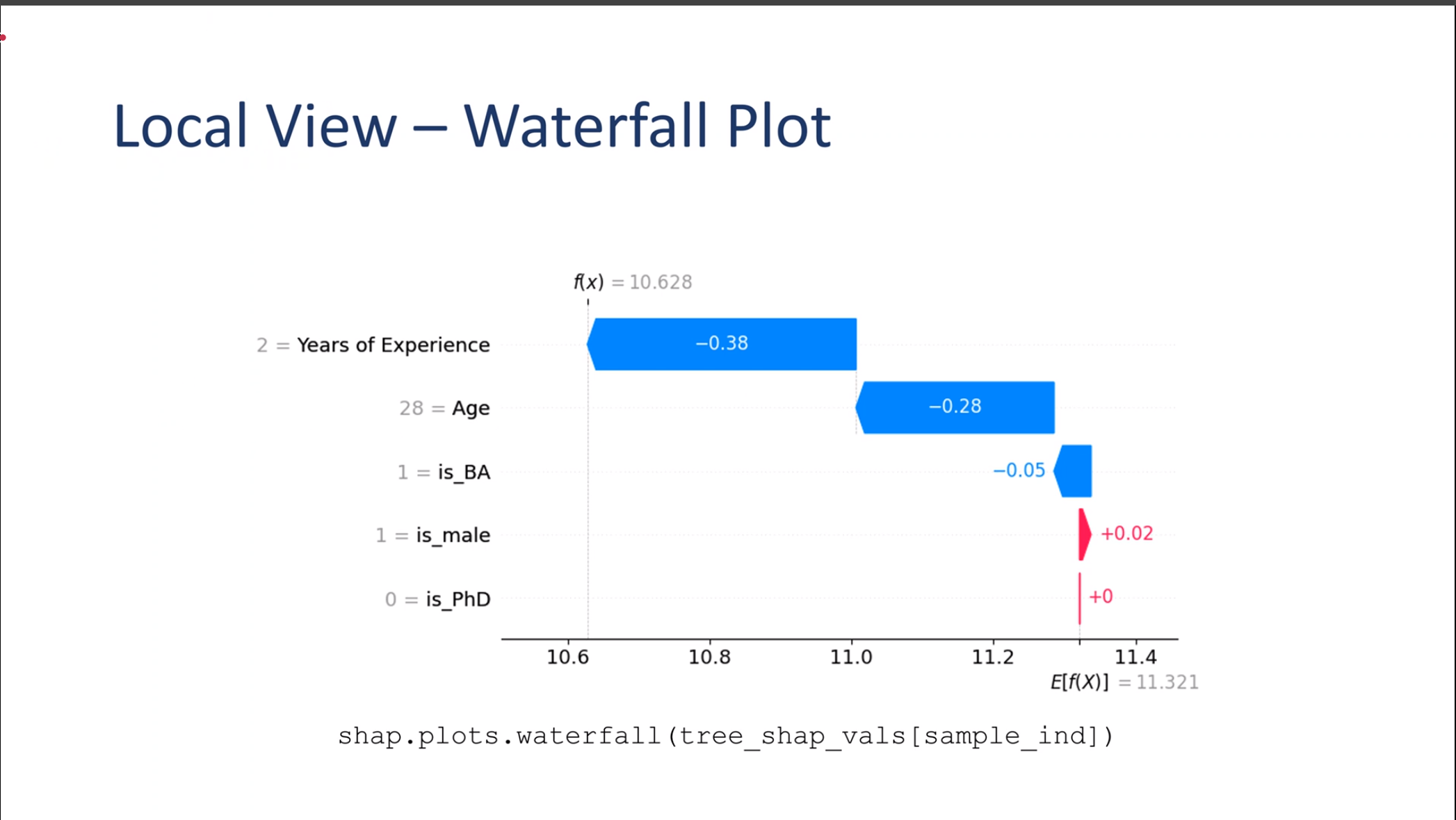
Local View – Waterfall Plot
Local Waterfall Plot
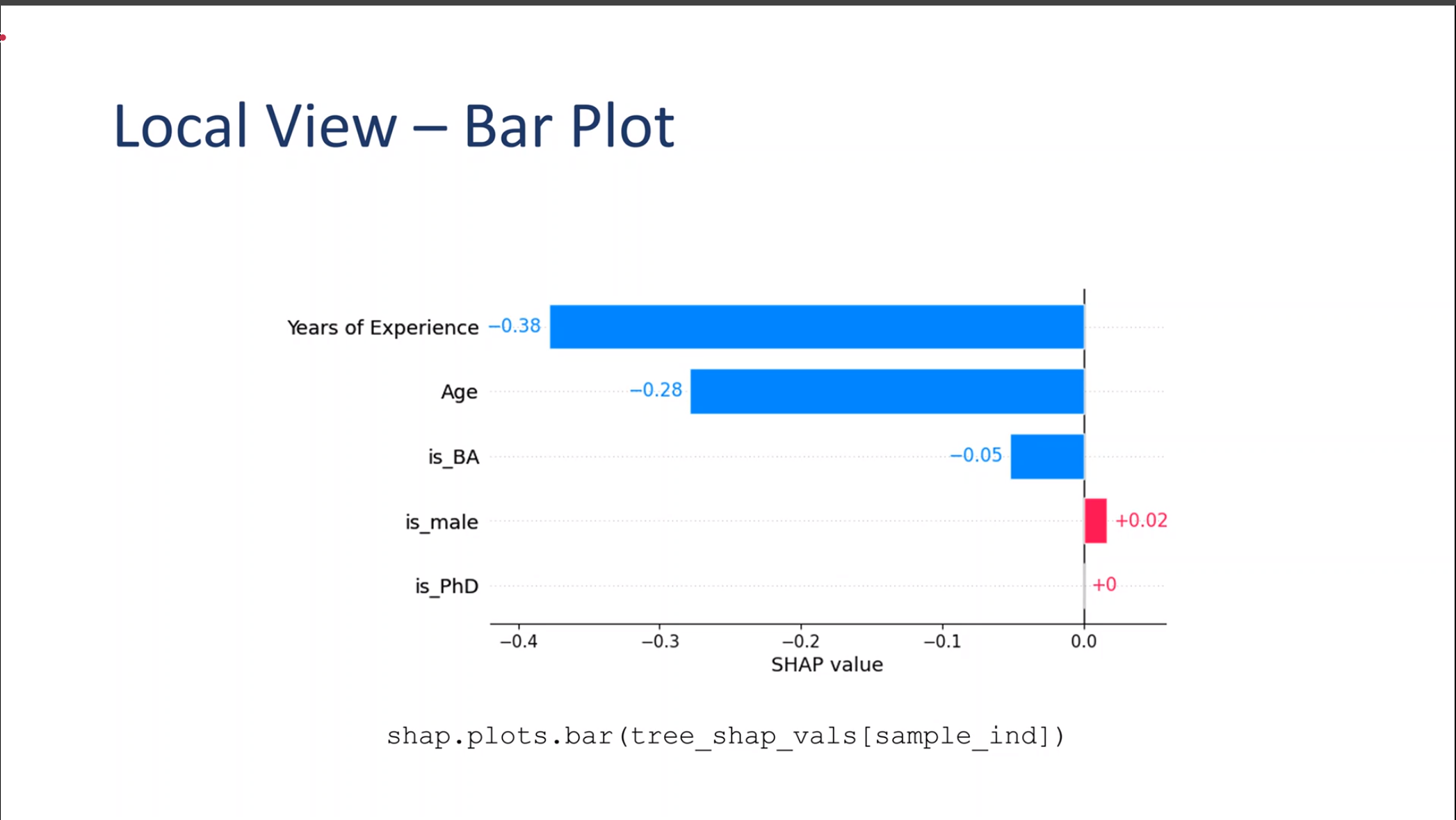
Local View – Bar Plot
Local Bar Plot
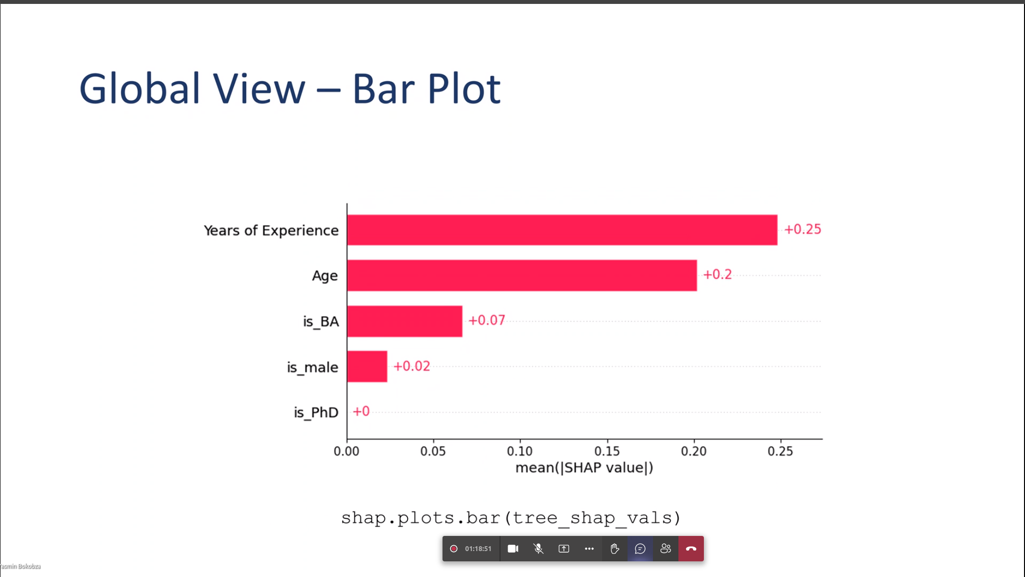
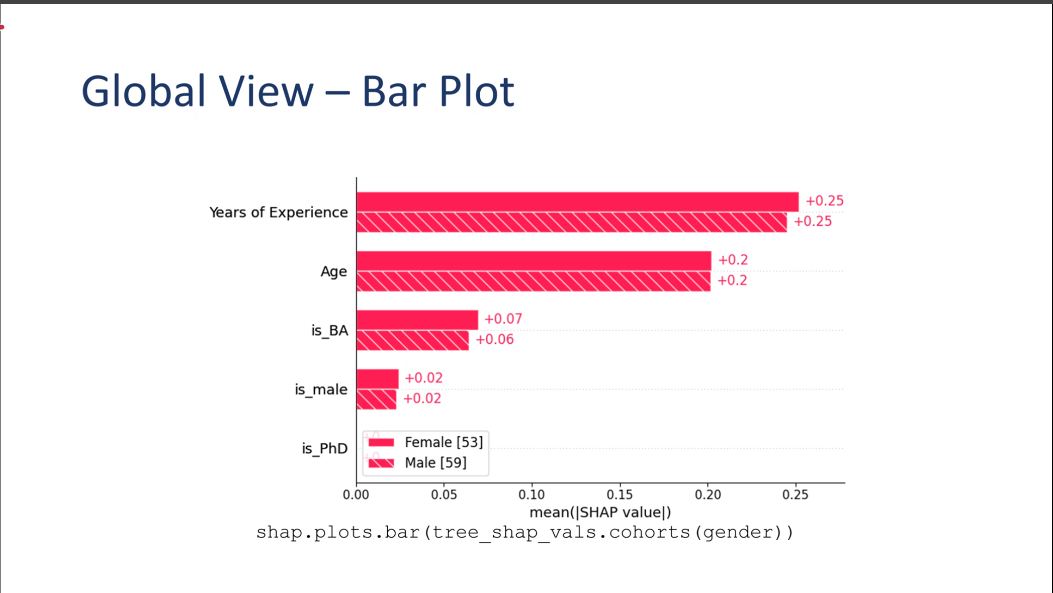
Global View – Bar Plot
Global Bar Plot
Global Bar Plot
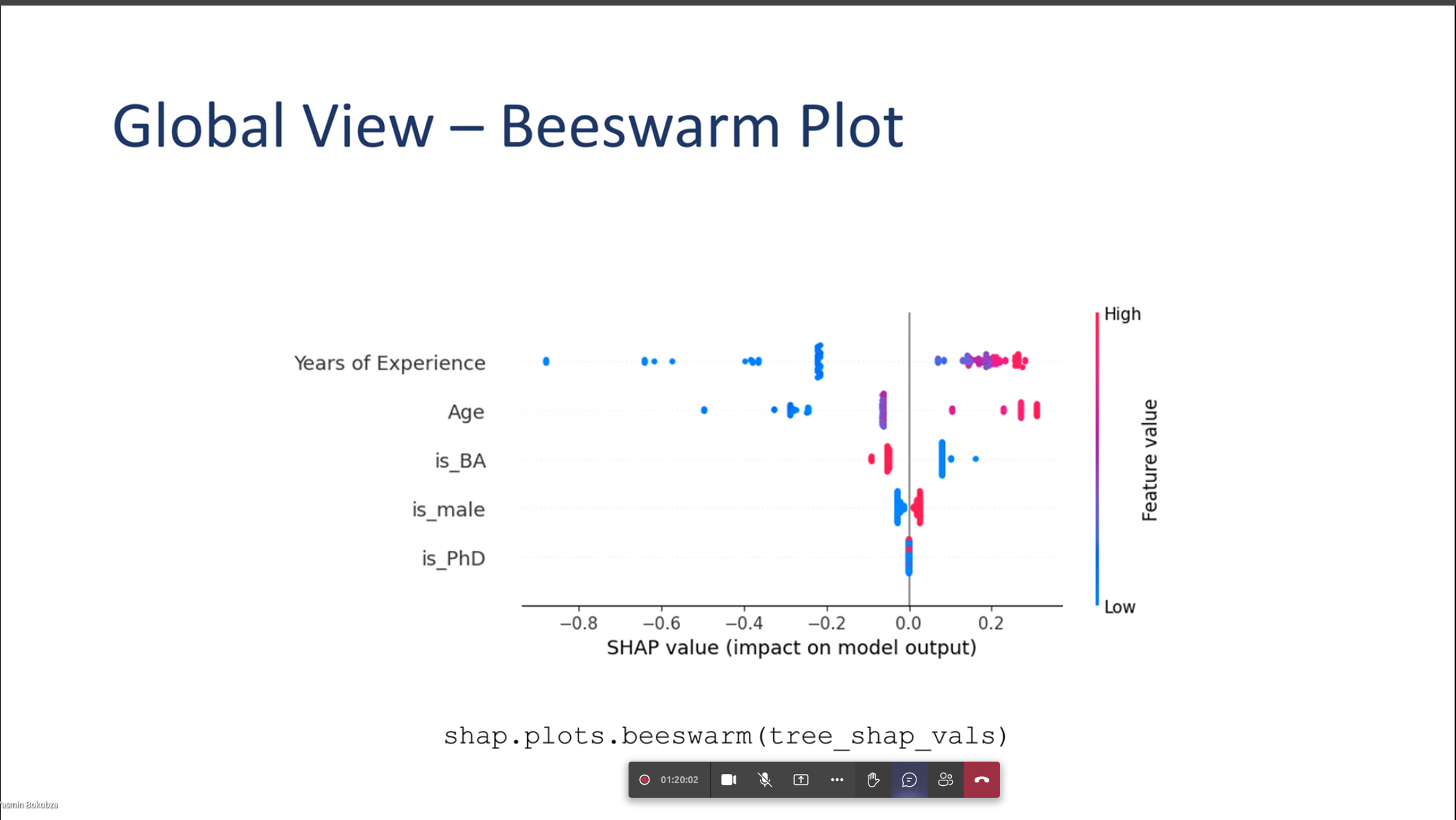
Global View – Beeswarm Plot
Global Beeswarm
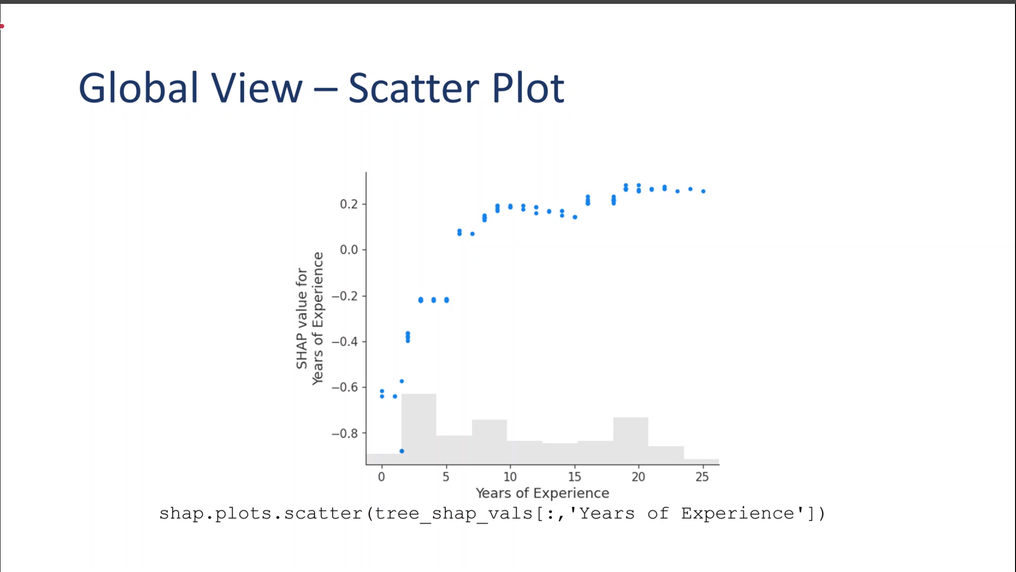
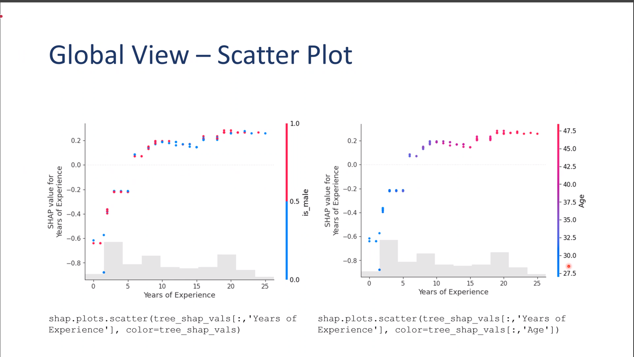
Global View – Scatter Plot
Global Scatter Plot
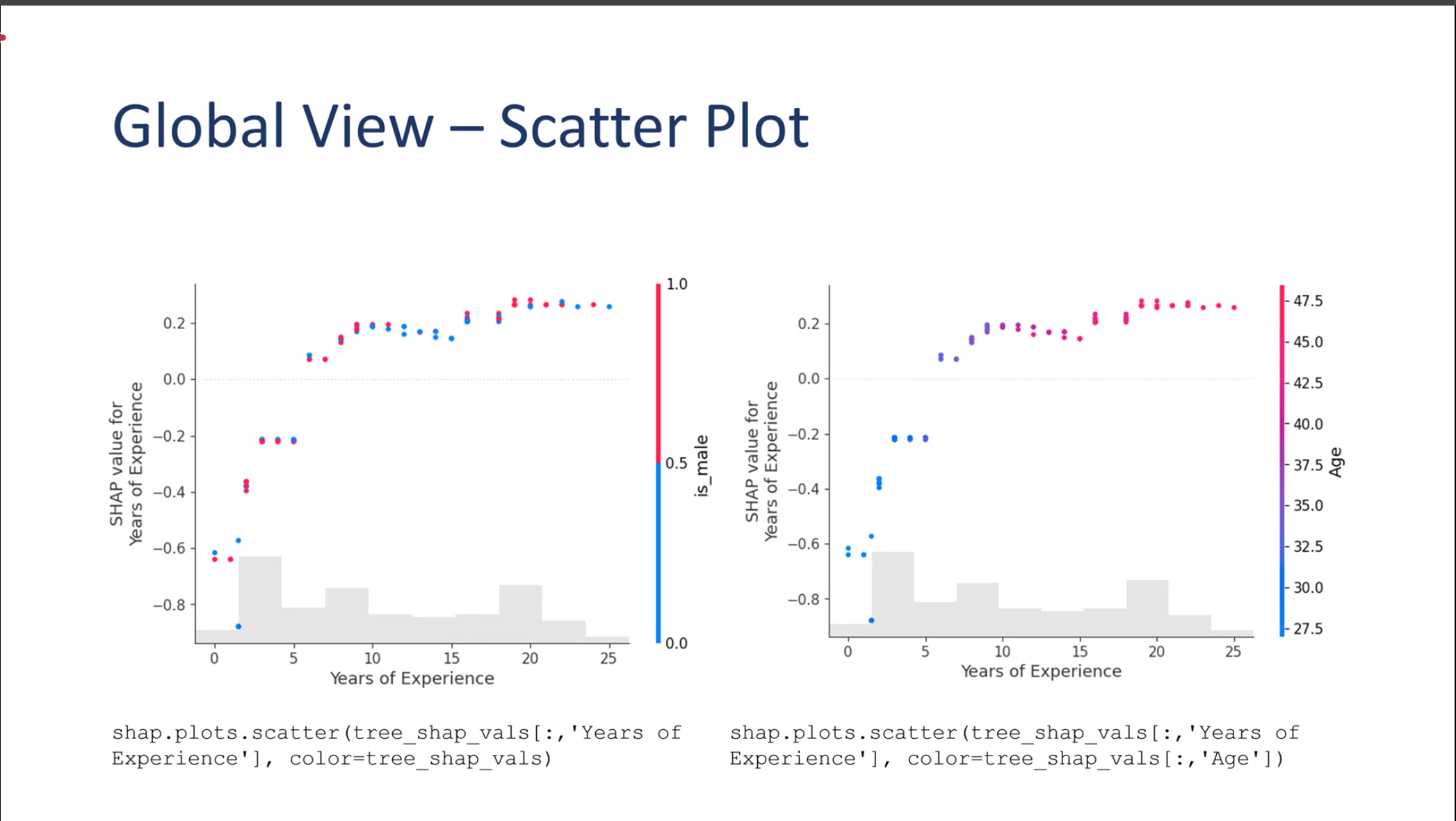
Global View – Scatter Plot
Globle Scatter Plot
Global View – Scatter Plot
Globle Scatter Plot
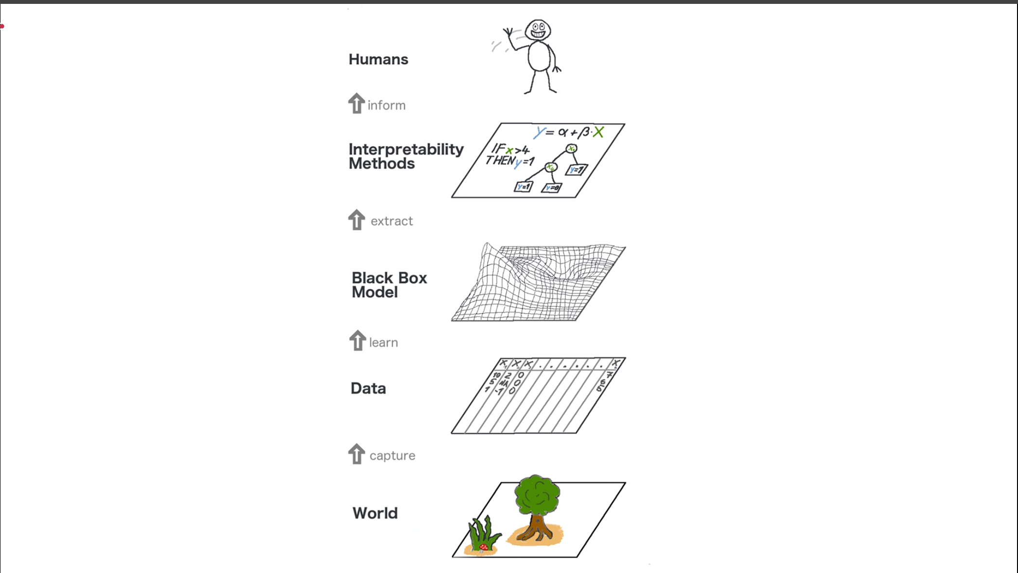
Model Hierarchy
Model Hierarchy
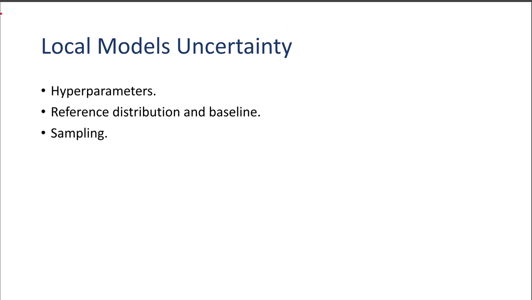
Local Uncertainty
Local Uncertainty
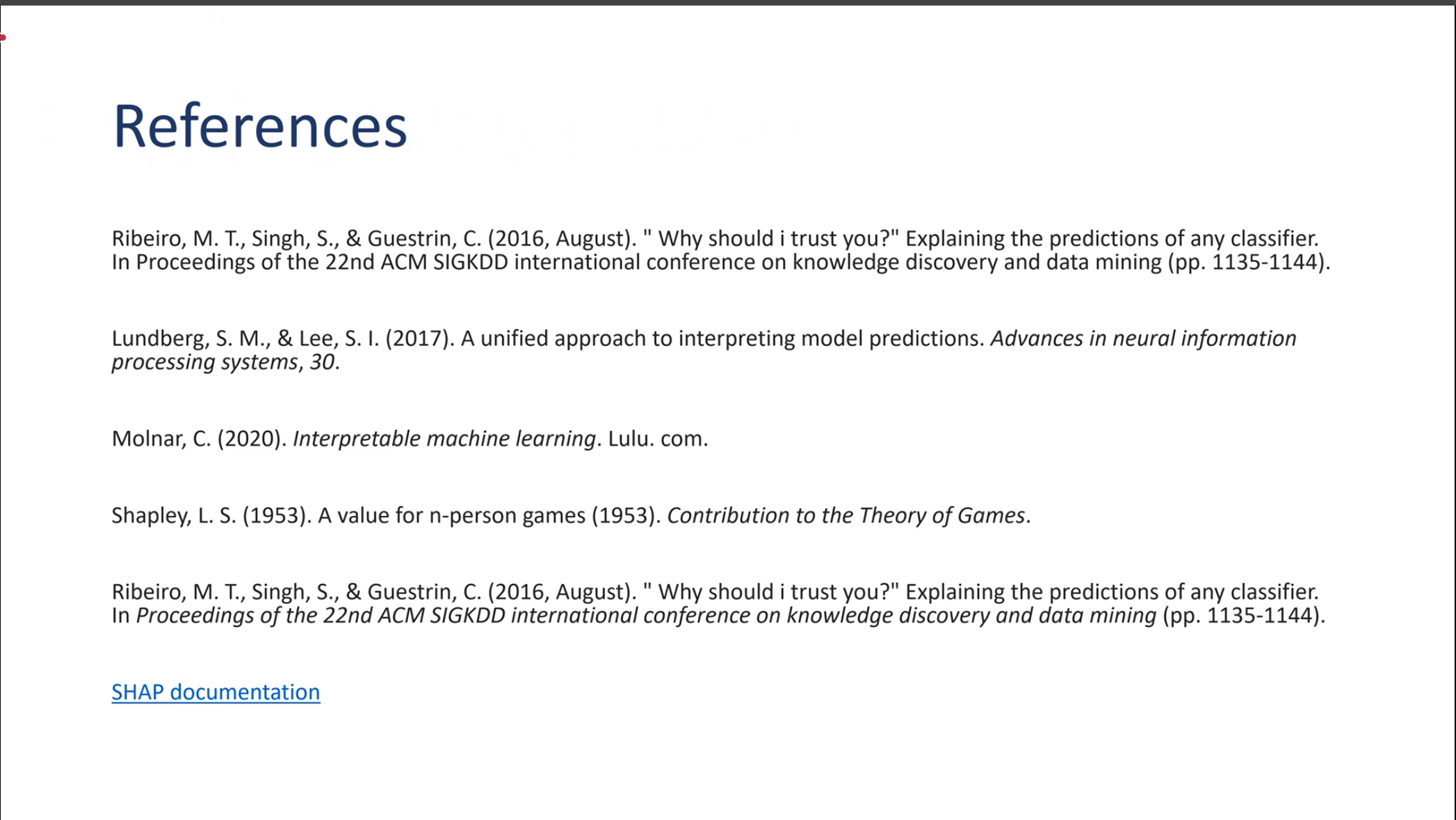
References
References
Conclusion
This course presented so much information it is easy to loose sight of some key point, so here are a few conclusions.
other approaches which include EDA.
using more transparent models e.g. regressions or statistical models.
by far the most prevalent approach in XAI is post hoc methods.
defined global and local explanations and noted their limitations.
What do we mean by explanations in XAI:
could be any number of visualization.
could be a simplified model. 💡 locally a complex manifold may look flat.
could be a ranking of the features by their contribution. 💡 SHAP and MIE
Goldstein, Alex, Adam Kapelner, Justin Bleich, and Emily Pitkin. 2013. “Peeking Inside the Black Box: Visualizing Statistical Learning with Plots of Individual Conditional Expectation.”Journal of Computational and Graphical Statistics 24: 44–65. https://api.semanticscholar.org/CorpusID:88519447.
Poyiadzi, Rafael, Kacper Sokol, Raúl Santos-Rodriguez, Tijl De Bie, and Peter A. Flach. 2019. “FACE: Feasible and Actionable Counterfactual Explanations.”CoRR abs/1909.09369. http://arxiv.org/abs/1909.09369.
Ribeiro, Marco Tulio, Sameer Singh, and Carlos Guestrin. 2016. “Why Should I Trust You?: Explaining the Predictions of Any Classifier.” In Proceedings of the 22nd ACM SIGKDD International Conference on Knowledge Discovery and Data Mining, 1135–44. KDD ’16. New York, NY, USA: Association for Computing Machinery. https://doi.org/10.1145/2939672.2939778.
Selvaraju, Ramprasaath R., Abhishek Das, Ramakrishna Vedantam, Michael Cogswell, Devi Parikh, and Dhruv Batra. 2016. “Grad-CAM: Why Did You Say That? Visual Explanations from Deep Networks via Gradient-Based Localization.”CoRR abs/1610.02391. http://arxiv.org/abs/1610.02391.
Zilke, Jan Ruben, Eneldo Loza Mencía, and Frederik Janssen. 2016. “DeepRED - Rule Extraction from Deep Neural Networks.” In IFIP Working Conference on Database Semantics. https://api.semanticscholar.org/CorpusID:10289003.
A depth 3 refression descision tree for the Salary DataSet
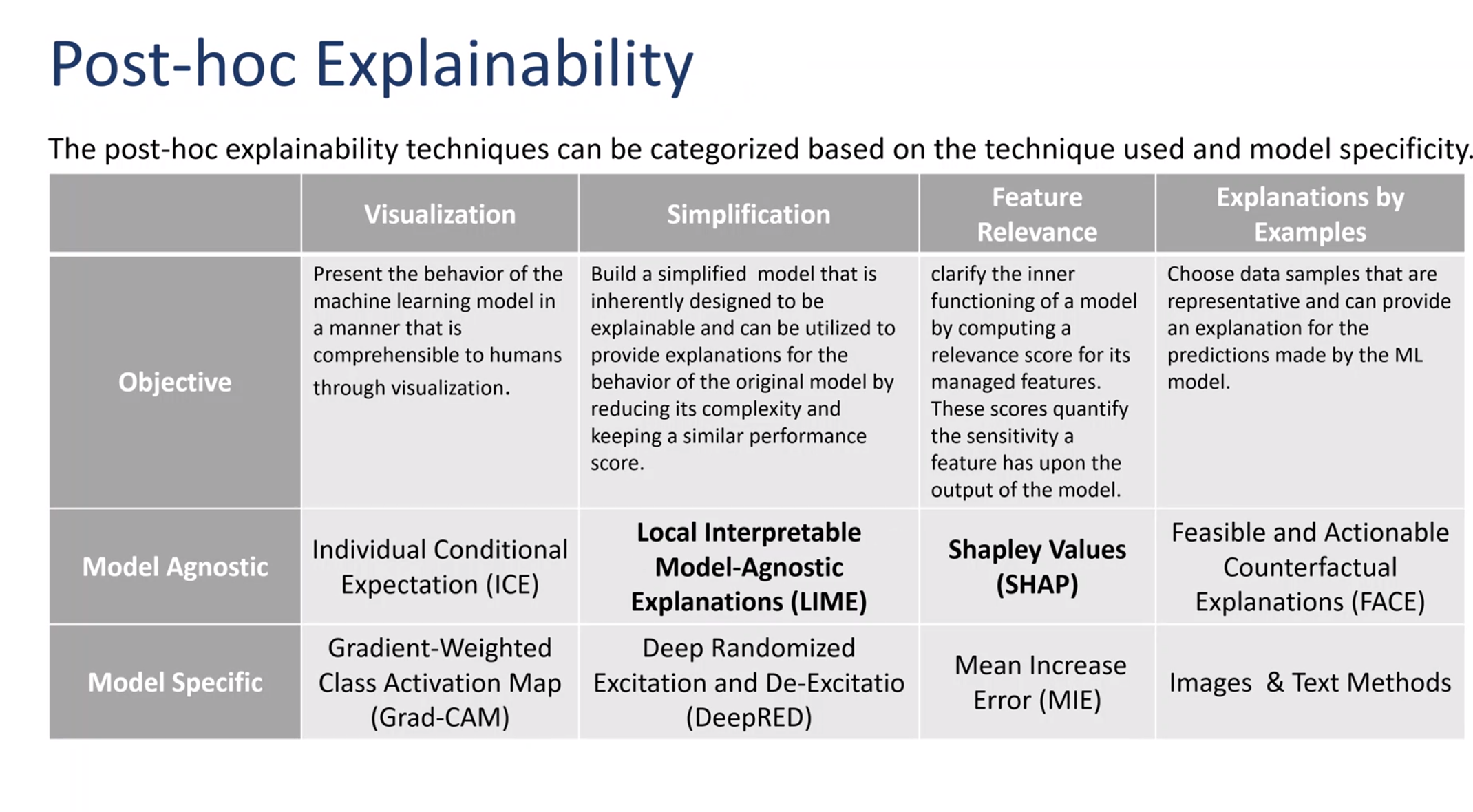
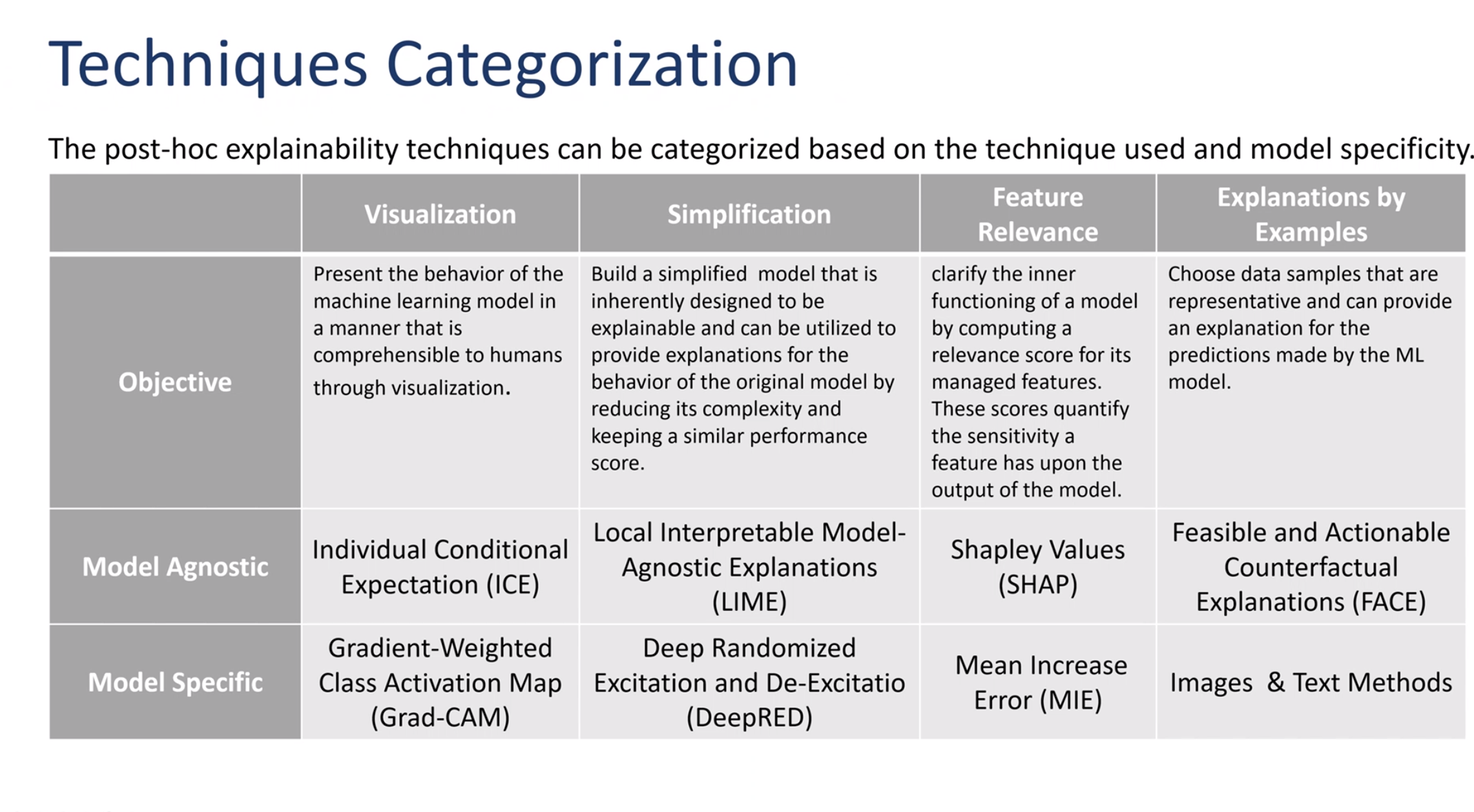 ## Post-hoc Explainability Table