Introduction
![]()
- We now start the third course in the reinforcement learning specialization.
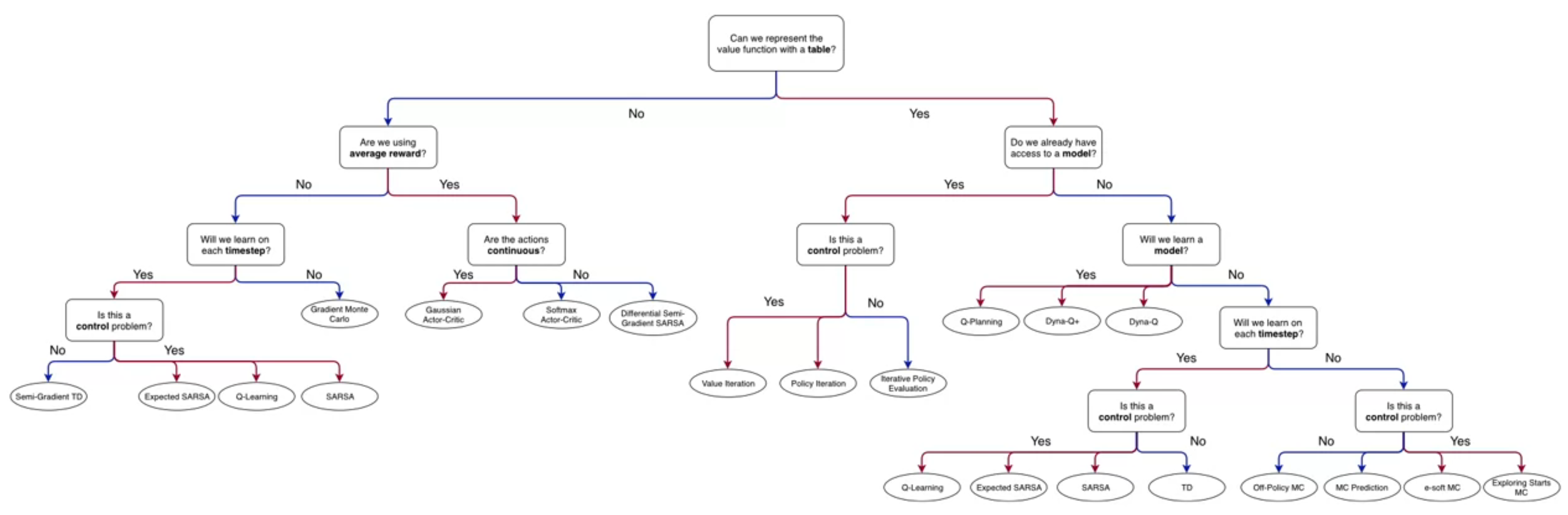
- In terms of the ?@fig-rl-chart we are on the left branch of the tree.
- This course is about prediction and control with function approximation.
- The main difference in this course is that will start consider continuous state spaces and action spaces which cannot be represented as tables.
- However many of the methods we will develop will be useful in handling large scale tabular problems as well.
- We will use methods from supervised learning but only online methods that can handle non-stationary data.
- The main differences are the use of weights to parameterize the value functions.
- The use of function approximation to estimate value functions and policies in reinforcement learning.
- Weights lead to using a loss function to estimate the value function.
- Minimizing the continuous loss function leads to Gradient descent and
- Using sampling leads to Stochastic gradient descent.
- The idea of learning weights rather than values is a key idea in this course.
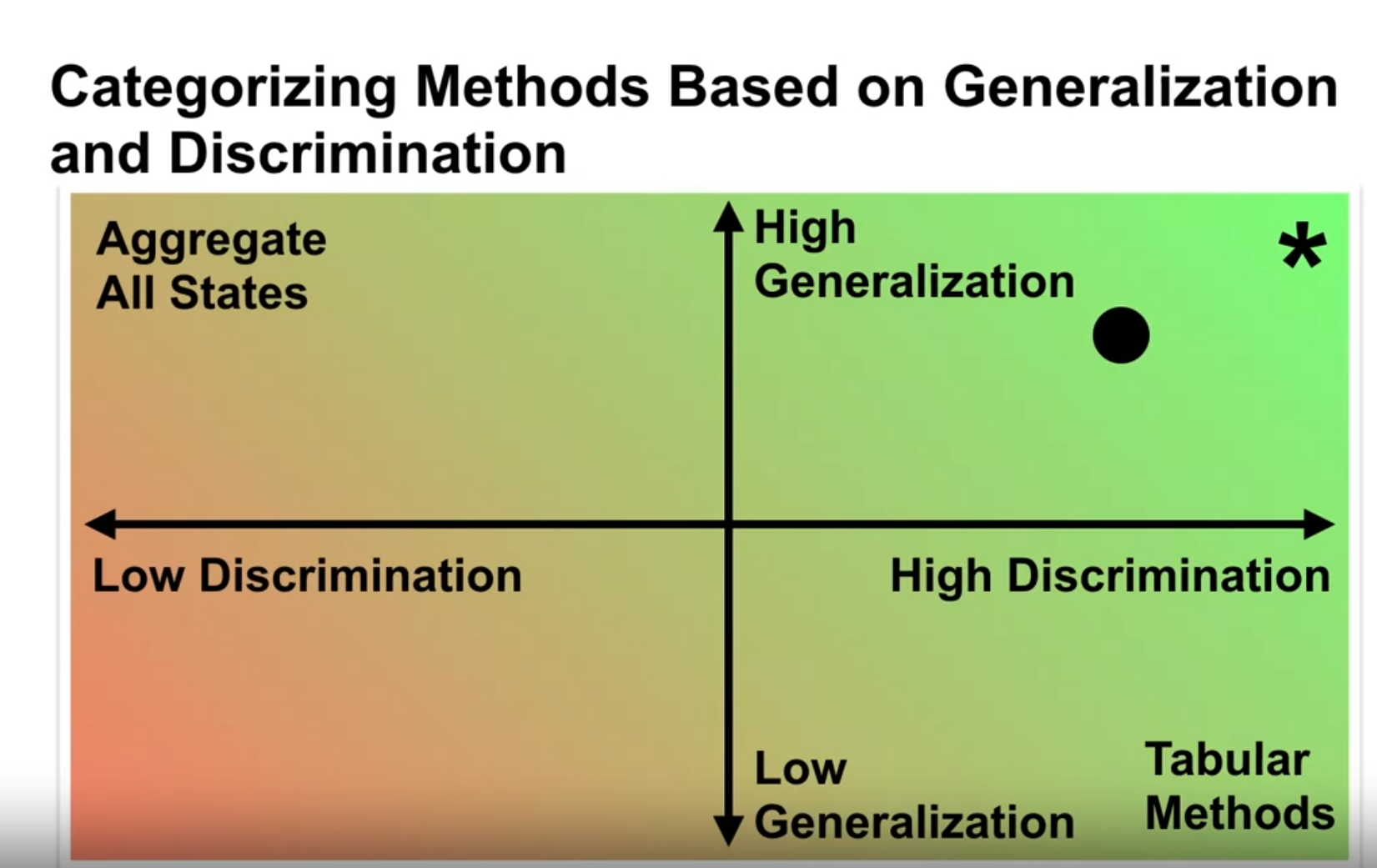
- The tradeoff between discrimination and generalization is also a key idea in this course.
- We will learn how to use function approximation to estimate value functions and policies in reinforcement learning.
- We will also learn how to use function approximation to solve large-scale reinforcement learning problems.
- We will see some simple linear function approximation methods and later
- We will see modern nonlinear approximation methods using deep neural networks.
I did not find the derivation of the SGD alg particularly enlightening and I have seen it several times. However the online setting is the best motivation for the use of SGD and makes perfect sense in the context of reinforcement learning. Minibatches are then a natural extension of this idea.
Lesson 1: Estimating Value Functions as Supervised Learning
In this lesson we will cover some important notation that will remain with us till the end of the course. Mathematically most of it is trivial, but it is important to understand the notation - otherwise the rest of the course will be hard to follow.
Moving to Parameterized Policies (video)
This video covers the first four learning objectives.
This video covers parameterized policies and how they can be used to approximate value functions. The idea is that using a table has some limitations/ The first is that the tables can be very large. For continuous states they can become infinite.
The second is that the tables can be very sparse and in a table we don’t generalize between states.
We see that we don’t really want functions that directly approximate the value function. We want functions that have some structure that we can learn.
This is called a parameterized function. The ideas is to use a weighted sum of the features of the state. This allows us to learn the weights and use them to approximate the value function. This is called linear function approximation. The way to get around this which is two fold. We first represent the salient properties of a states into features.
Then we use weights to combine these features to approximate the value function. This is called linear function approximation.
More generally we can use non linear parameterized functions to approximate value functions.
Adam shows that is the features are not picked wisely we may not be able to discriminate between states - out function for one state will be the same as for another dissimilar state. Learning about one will make us forget what we learned about the other. This is called bias. On the other hand if we have too many features we may not be able to generalize between states. This is called variance. The goal is to balance between bias and variance.
Understanding parameterized functions
- In the previous courses we represented value functions as tables or arrays:
- For V(s) we had an array of size |S|,
- For Q(s,a) we had an array of size |S| \times |A|. This becomes impractical as |S| \rightarrow \infty. We can use parameterized functions to approximate value functions. This is called function approximation.
- Linear value function approximation is a simple and popular method.
- We represent the value function as a linear combination of features:
\hat{v}(s, \mathbb{w}) \approx v_\pi(s) \qquad \tag{1}
- where:
- \hat{v}() is the approximate value function
- \mathbf{w} is a weight vector
- for example:
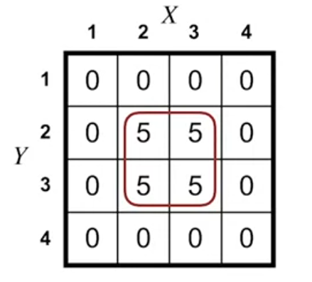
Linear value function approximation
- We can write the approximate value function as a linear combination of features:
\hat{v}(s, \mathbb{w}) \dot = w_1 X + w_2 + Y \qquad \tag{2}
- where:
- X and Y are features of the state s
- w_1 and w_2 are the weights of the features
- now learning becomes finding better weights that parameterize the value function.
finding the weights that minimize the error between the approximate value function and the true value function:
Tabular case is a special case of linear value function approximation
\begin{align*} \hat{v}(s, \mathbb{w}) & \dot = \sum w_i x_i(s) \newline & = <\mathbf{w}, \mathbf{x}(s)> \qquad \end{align*}
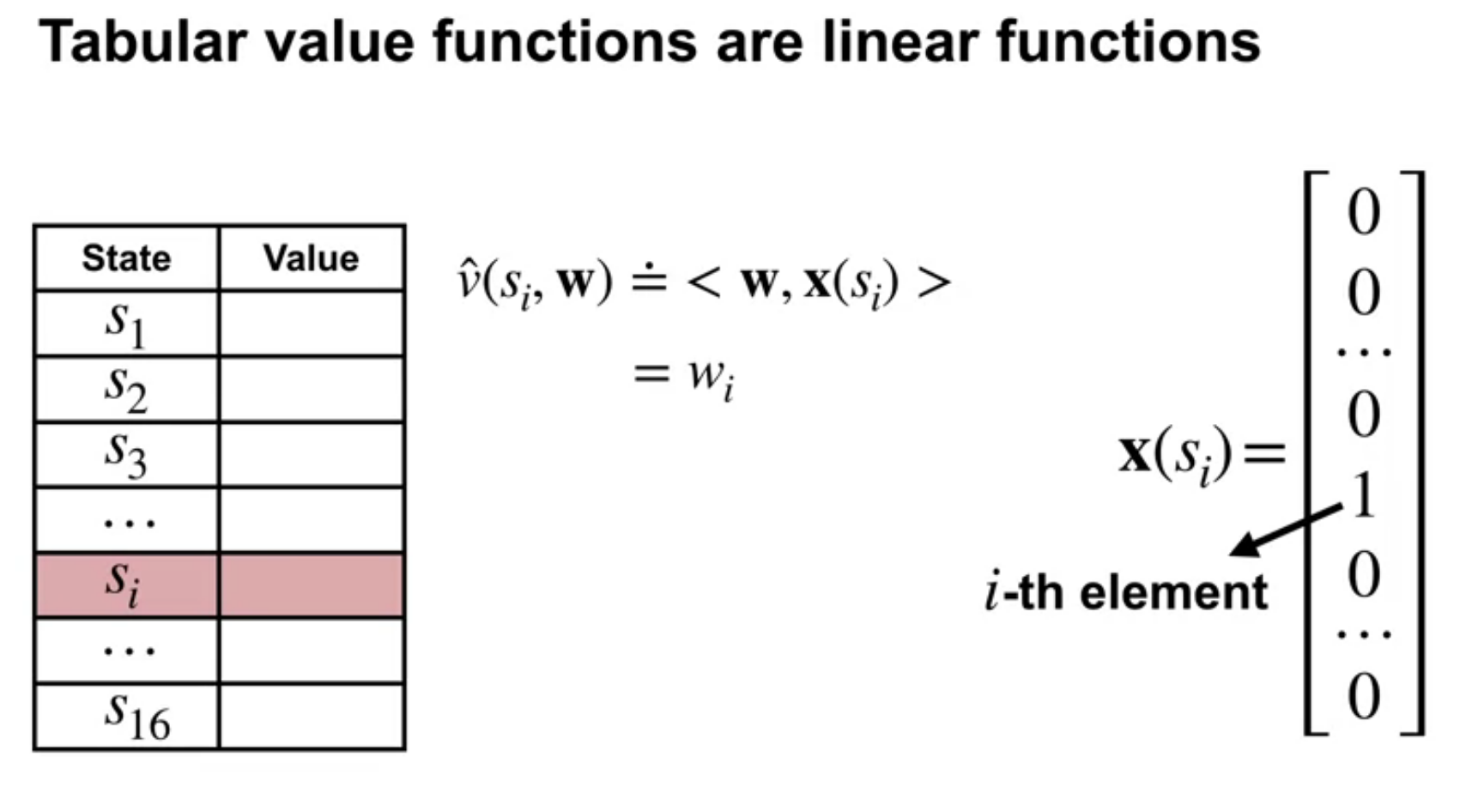
- here:
- \mathbf{w} is a weight vector
- \mathbf{x}(s) is a feature vector that is 1 in the i-th position and 0 elsewhere.
- linear value function approximation is a generalization of the tabular case.
- limitations of linear value function approximation:
- the choice of features limits the expressiveness of the value function.
- it can only represent linear relationships between the features and the value function.
- it can only represent a limited number of features.
- so how are tabular functions a special case of linear value function approximation?
- we can see from the figure that all we need is use one hot encoding for the features. Then the weighted vector will be the same as the value function in the table.
There are many ways to parameterize an approximate value function
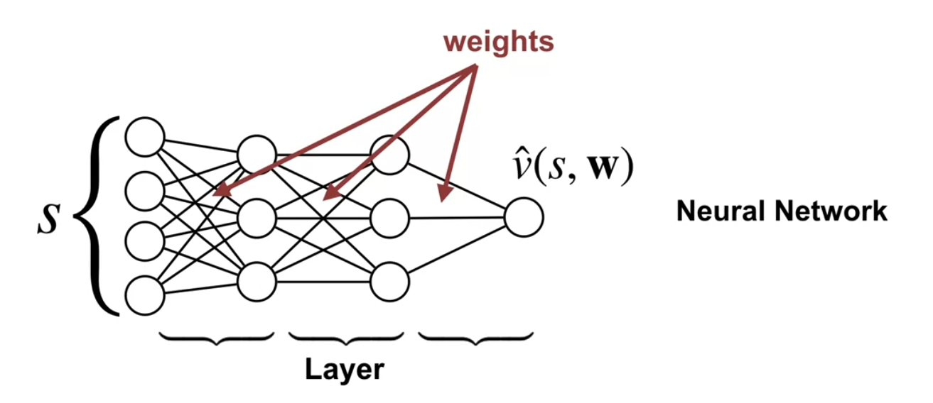
- We can use different types of functions to approximate the value function:
- one hot encoding
- linear functions
- tile coding
- neural networks
Generalization and Discrimination (video)
In this video Martha covers the next three learning objectives. The video is about:
- Generalization - using knowledge (V,Q,Pi) about similar states.
- Discrimination - being able to distinguish between different states.
Understanding generalization and discrimination
- Generalization:
- the ability to estimate the value of states that were not seen during training.
- in the case of policy evaluation, generalization is the ability of updates of value functions in one state to affect the value of other states.
- in the tabular case, generalization is not possible because we only update the value of the state we are in.
- in the case of function approximation, we can think of generalization as corresponding to an embedding of the state space into a lower-dimensional space.
- Discrimination: the ability to distinguish between different states.
How generalization can be beneficial
- Generalization can be beneficial because:
- It allows us to estimate the value of states that are similar to states seen during training.
- This includes states that were not seen during training.
- It allows us to estimate the value of states that are far from states seen during training. (So long as they are similar in terms of the features we are using to approximate the value function)
Why we want both generalization and discrimination from our function approximation
- We want both generalization and discrimination from our function approximation because:
- generalization allows us to estimate the value of states that were not seen during training.
- discrimination allows us to distinguish between different states.
- generalization allows us to estimate the value of states that are similar to states seen during training.
- discrimination allows us to estimate the value of states that are far from states seen during training.
We hear a lot about function approximation and gradient methods having a bias or high variance. I tracked this from wikipedia and statistical learning. While it makes sense for a Bayesian regression I’m not sure that it is quite correct for RL. Unfortunately I don’t have a better explanation, though reviewing this policy gradient lecture might be helpful
- an important result called the bias-variance tradeoff:
- Bias is the error introduced by approximating a real-world problem, which may be extremely complicated, by a much simpler model. This means that since we cannot discriminate between different states that share weights for the same feature vector we have errors we characterize as bias.
- High bias corresponds to underfitting in our model.
- Variance is the opposite issue arising from having more features than we need to discriminate between states. This means that updating certain weights will affect only some of these related states and not others. This type of error is called variance and is also undesirable.
- High variance corresponds to overfitting in our model which can be due to our model fitting the noise in the data rather than the underlying signal.
- In general for a model there is some optimal point where the bias and variance are balanced. Going forward from that point we observe a trade off between bias and variance so we need to choose one or the other.
- This choice is usually governed by business realities and the nature of the data or the problem we are trying to solve.
Framing Value Estimation as Supervised Learning (video)
In this video we cover the next two learning objectives. Martha has a good background in supervised learning and she explains how many parts of RL can be framed as supervised learning problems.
Things we like to learn in RL in this course:
- Value fn approximation (V)
- Action fn values (Q)
- Policies (Pi)
In reality we may want to learn other things as well which can be framed as supervised learning problems:
- State representations - i.e. better features (CNNs, RNNs, etc)
- Models of Dynamics i.e. Transition probabilities (P)
- Reward precesses (R) What is a good reward function? How do we learn it? This is an inverse reinforcement learning problem. It is ill posed because there are many reward functions that can explain the data. We need to find the simplest one that explains the data. This is intertwined with learning internal motivations and goals. c.f. Satinder Singh’s work on intrinsic motivation.
- Generalized Value functions (Gvfs) c.f. Martha and Adam White’s work on GVFs.
- Options (Spatial or Temporal Aggregations of actions) c.f. Doina Precup’s work on options and semi-markov decision processes.
Even more things that we might want to learn in RL that might be framed as supervised learning problems:
- Approximate/Compressed policies for sub goals AKA heuristics
- Fully Pooled policies (all states are the same) - Think random uniform policy
- Partial pooled policies, (some states are the same)
- Unpooled policies (all states are different - tabular setting)
- Priors for Policies
- Hierarchies of options - Think Nethack
- Beliefs about policies
- Beliefs about other agents (theory of mind)
- Beliefs about the environment.
- Causal models of the environment
- what can we influence and what can’t we influence.
- Coordination and communication with other agents c.f. work by Jakob Foerster, Natasha Jacques, and Marco Baroni on emergent communication.
- What part of communication is cheap talk
- What part of communication is credible
How value estimation can be framed as a supervised learning problem
The problem of policy evaluation in reinforcement learning can be framed as supervised learning problem
- In the case of Monte Carlo methods,
- the inputs are the states and
- the outputs are the returns G.
- In the case of TD methods,
- the inputs are the states and
- the outputs are the one step bootstrapped returns. U_t \dot=R_{t+1} + \gamma \hat{v}(S_{t+1}, \mathbf{w})
- In the case of Monte Carlo methods,
Not all function approximation methods are well suited for reinforcement learning
In principle, any function approximation technique from supervised learning can be applied to the policy evaluation task. However, not all are equally well-suited. – Martha White
- in RL the agent interacts with the environment and generates data, which corresponds to the online setting in supervised learning.
- When we want to use supervised learning we need to choose a method that is well suited for the online setting which can handle
- non-stationary data.
- non-stationary and correlated data (which is the case in RL).
In fact much of the learning in RL is about learning such correlations and quickly adapting to non-stationary in the environment.
In TD learning the target depends on w but in supervised learning the target is fixed and given.
Lesson 2: The Objective for On-policy Prediction
The Value Error Objective (Video)
In this video Adam White covers the first two learning objectives of the unit.
The main subject about using the mean squared error as a loss for the approximate value function.
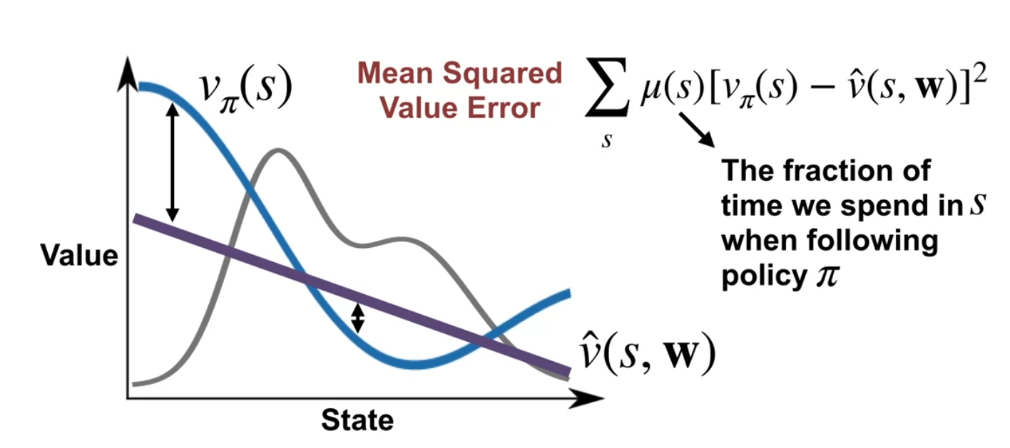
we get a sequence of (S_1,v_{\pi}(S_1) ),(S_2,v_{\pi}(S_2) ),(S_3,v_{\pi}(S_3) ), \ldots and we want to approximate the value function . We can track how well we are approximating v_{\pi}(s) by using \hat{v}(s,\mathbb{w}). The difference can be positive or negative so if we average it the sum will tend to cancel out. If we square the error we get a positive number we have a much better estimate of the error. And if normalize it by taking the mean we can get use it to compare runs of different lengths. This is called the mean squared error.
It turns out that this is not enough for RL and we need to take a weighted average using the state distribution \mu(s). This is because we care more about some states than others. The state distribution is the long run probability of visiting the state s under the policy \pi. This weighted average is called the mean squared value error.
In the optimization literature the loss function is called the objective function. This is because we are trying to optimize the weights of the function to minimize the loss. So we will often hear the term objective function or just objective. Life is simpler if we recall that this is just a loss function for a supervised learning problem.
A related point is that if we want to optimize our approximate value we can swap the with a different loss function or with a different approximation function and the outcome should remain the same, at least under certain conditions. This is how we can switch from the mean squared value error objective to the Monte Carlo objective and then to the TD learning objective.
Understanding the mean-squared value error objective for policy evaluation
- An idealized Scenario:
- input: \{(S_1, v_\pi(S_1)), (S_2, v_\pi(S_2)), \ldots, (S_n, v_\pi(S_n))\}
- output: \hat v(s,w) \approx v_\pi(s)
- however in reality we may get some some error in the approximation.
- this could be due to our choice of the approximation.
- but initially we just don’t have good weights - to fit the data.
- What we need is a way to measure the error in the approximation.
- Also we may care more about some states than others and we can encode this using the state distribution \mu(s).
- The mean-squared value error objective for policy evaluation is to minimize the mean-squared error between the true value function and the approximate value function:
\overline{VE} = \sum_{s\in S}\mu(s)[v_\pi(S) - \hat{v}(S, \mathbf{w})]^2 \tag{3}
- where:
- \overline{VE} is the mean-squared value error
- \mu(s) is the state distribution
- v_\pi(s) is the true value of state s
- \hat{v}(s, \mathbf{w}) is the approximate value of state s with weights \mathbf{w}
- the goal is to find the weights that minimize the mean-squared value error.
Explaining the role of the state distribution in the objective
- The state distribution \mu(s) is the long run probability of visiting the state s under the policy \pi.
- This makes more sense if our markov chain is ergodic - i.e. we can reach any state from any other state by following some transition trajectory.
- The state distribution is important because it determines how much we care about the error in each state.
- The state distribution is usually unknown, and hard to estimate as it has complex dependencies on the policy and the environment.
- We will later see a result that shows how we can avoid the need to know the state distribution.
- In the diagram we see that the state distribution is a probability distribution over the states of the MDP and that there is little probability mass of visiting states at the edges of the state space.
- The mean square error has less impact in these low probability states.
The idea behind gradient descent and stochastic gradient descent
- Gradient descent is an optimization algorithm that uses the gradient to find a local minimum of a function.
- The gradients points in the direction of the steepest ascent of the function and our objective is to minimize the mean squared error we move in the opposite direction.
- Hence the name gradient descent.
- The gradient of the mean-squared value error with respect to the weights \mathbf{w} is given by:
w \dot = \left [ \begin{matrix} w_1 \\ \vdots \\ w_d \end{matrix} \right ] \qquad \nabla f = \left [ \begin{matrix} \frac{\partial f}{\partial w_1} \\ \vdots \\ \frac{\partial f}{\partial w_d} \end{matrix} \right ] \qquad
- for a linear function:
\hat{v}(s, \mathbf{w}) = \sum \mathbf{w}^T \mathbf{x}(s) \\ \frac{\partial \hat{v}(s, \mathbf{w})}{\partial w_i} = \mathbf{x_i}(s) \\ \nabla \hat{v}(s, \mathbf{w}) = \mathbf{x}(s) \qquad \tag{4}
- we can write the update rule for the weights as:
w_{t+1} \dot= w_t - \alpha \nabla J(\mathbf{w_t}) \qquad \tag{5}
- Stochastic gradient descent is a variant of gradient descent that uses a random sample of the data to estimate the gradient.
- Stochastic gradient descent uses mini-batches of data to estimate the gradient, which makes it computationally efficient and reduces the variance of the gradient estimate.
- In practice we will use variants like:
- Adam - which adapts the learning rate based on the gradient.
- RMSProp - which uses a moving average of the squared gradient.
- Adagrad - which uses a different learning rate for each parameter.
- SGD - which uses a fixed learning rate.
Gradient descent converges to stationary points
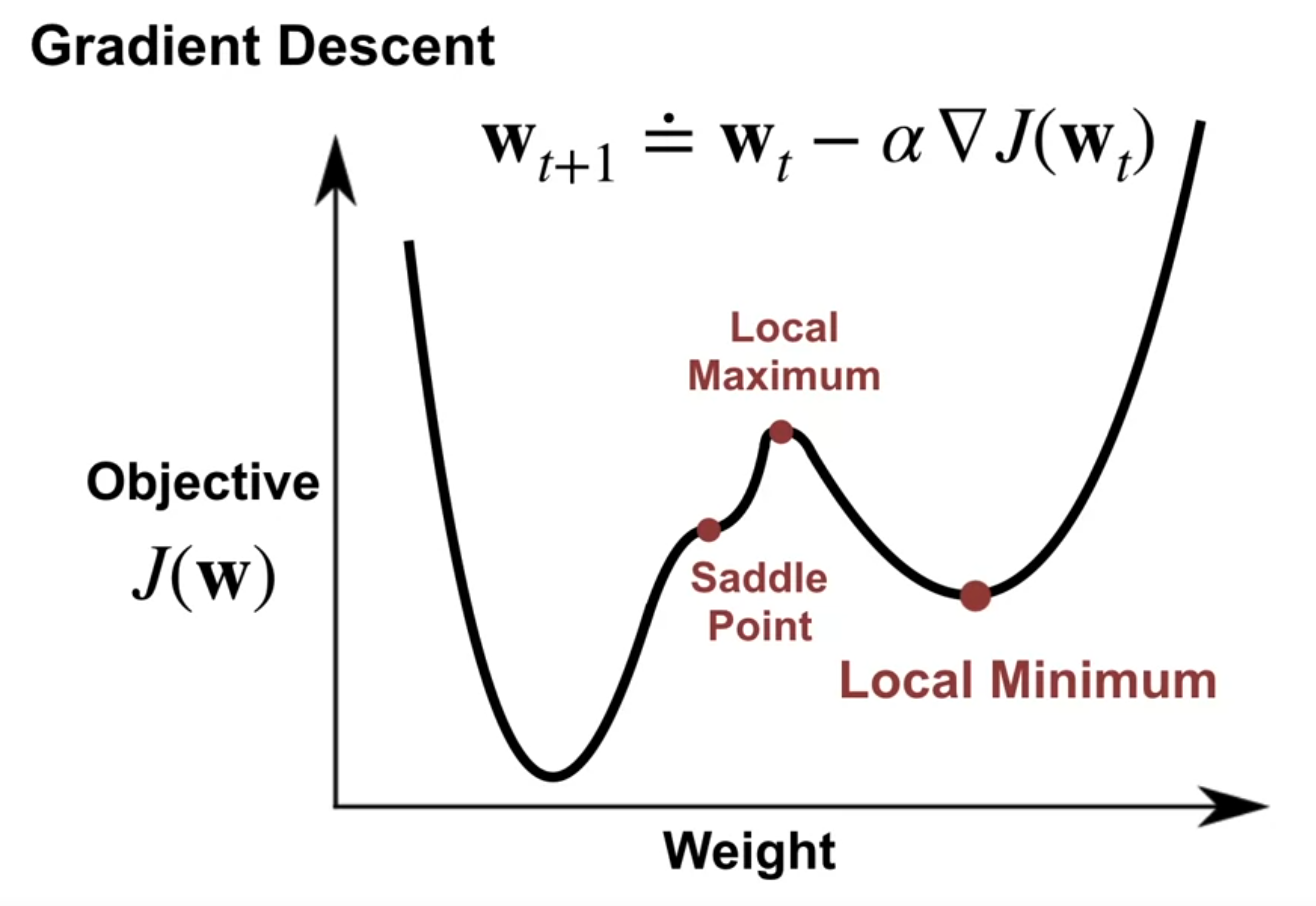
- Gradient descent converges to stationary points because the gradient of the mean-squared value error is zero at the minimum.
- Gradient descent can get stuck in a local minima, so it is important to use a good initialization and learning rate.
- Stochastic gradient descent can escape a local minima because it uses a random sample of the data to estimate the gradient.
- In general the optimizer is not guaranteed to find the global minimum of the function - just a local minima
How to use Gradient descent and Stochastic gradient descent to minimize the value error
\begin{align*} \nabla J(\mathbf{w}) & = \nabla \sum_{s\in S} \mu(s)[v_\pi(s) - \hat{v}(s, \mathbf{w})]^2 \qquad \qquad \hat{v}(s, \mathbf{w}) = <\mathbf{w},\mathbf{x}(s)>\newline & = \sum_{s\in S} \mu(s) \nabla [v_\pi(s) - \hat{v}(s, \mathbf{w})]^2 \qquad \qquad \nabla \hat{v}(s, \mathbf{w}) = \mathbf{x}(s)\newline & = \sum_{s\in S} \mu(s) 2 [v_\pi(s) - \hat{v}(s, \mathbf{w})]\nabla \hat{v}(s, \mathbf{w}) \end{align*} \qquad
Stochastic Gradient Descent
If we have a sample of states s_1, s_2, \ldots, s_n observed by following pi
we can write the update rule for a pair of weights as:
w_{t+1} \dot= w_t + \alpha [v_\pi(S_1) - \hat{v}(s_1, \mathbf{w_1})]\nabla \hat{v}(s, \mathbf{w}) \qquad \tag{6}
This allows us to decrease the error in the value function by making updates for one state at a time and moving the weights in the direction of the negative gradient. By making this type of update we might increase the error occasionally but in the long run we will decrease the error.
This updating approach is called stochastic gradient descent, because it only uses a stochastic estimate of the gradient. In fact, the expectation of each stochastic gradient equals the gradient of the objective. You can think of this stochastic gradient as a noisy approximation to the gradient that is much cheaper to compute, but can nonetheless make steady progress to a minimum – Martha White
we have here one issue - we don’t know the true value of the policy v_pi(s_1), how do we get around this?
one option is to replace the true value with an estimate, one option is to use the return from the state s_1.
recall that
v_\pi(s) = \mathbb{E}[G_t \mid S_t = s] \qquad
so we can substitute the true value with the return from the state s_1.
\begin{align*} w_{t+1} & \dot= w_t + \alpha [v_\pi(S_1) - \hat{v}(s_1, \mathbf{w_1})]\nabla \hat{v}(s, \mathbf{w}) \qquad \\ & \dot = w_t + \alpha [G_1 - \hat{v}(s_1, \mathbf{w_1})]\nabla \hat{v}(s, \mathbf{w}) \qquad \end{align*} \tag{7}
The gradient Monte Carlo algorithm for value estimation
We now have a way to update the weights of the value function using the gradient of the mean-squared value error. Which allows us to present the gradient Monte Carlo algorithm for value estimation.
- The Gradient Monte Carlo algorithm is a policy evaluation algorithm that uses stochastic gradient descent to minimize the mean-squared value error.
How state aggregation can be used to approximate the value function
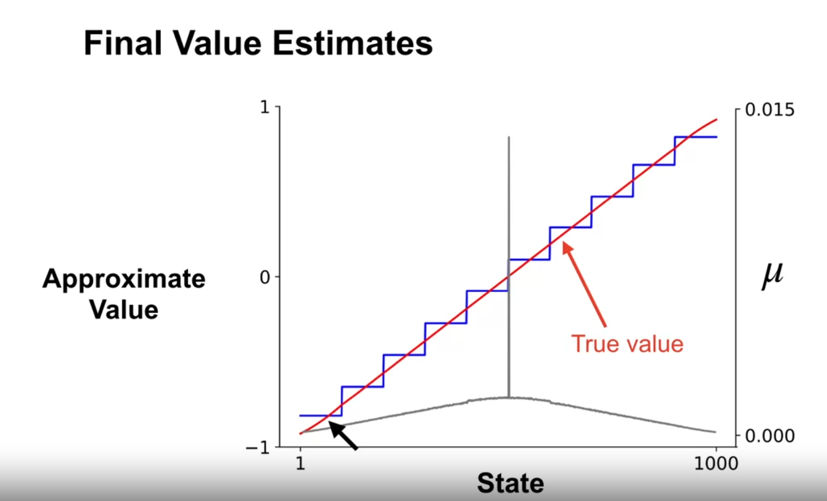
- State aggregation
- is a method for reducing the dimensionality of the state space by grouping similar states together.
- can be used to approximate the value function by representing each group of states as a single state.
- can be used to reduce the number of parameters in the value function and improve generalization.
- the example used a 1000 state MDP with 10 groups of 100 states each.
- left and right jump left 1-100 states and right 1-100 states.
- if they pass the terminal state they get to the terminal state.
- state aggregation is a way to reduce the number of parameters in the value function by grouping similar states together.
- it is an example of linear function approximation.
- there is one feature for each group of states.
- the weights are updated using the gradient of the mean-squared value error.
w \leftarrow w + \alpha [G_t - \hat{v}(S_t, \mathbf{w})] \nabla \hat{v}(S_t, \mathbf{w})
and the gradient of the approximate value function is given by:
\nabla \hat{v}(S_t, \mathbf{w}) = \mathbf{x}(S_t)
which is either 1 or 0 depending on the group of states.
Applying Gradient Monte-Carlo with state aggregation
- Gradient Monte Carlo with state aggregation is a policy evaluation algorithm that uses state aggregation to approximate the value function.
- The algorithm works as follows:
Lesson 3: The Objective for TD
The TD-update for function approximation
- recall the Monte Carlo update rule:
w \leftarrow w + \alpha [G_t - \hat{v}(S_t, \mathbf{w})] \nabla \hat{v}(S_t, \mathbf{w})
- we can use other targets for the update rule than the return G_t.
- we can replace the return with any estimate of the value of the next state.
- we can call this target U_t and if it is unbiased it converge to a local minimum of the mean squared value error.
- we can use the one step bootstrapped return:
U_t \dot=R_{t+1} + \gamma \hat{v}(S_{t+1}, \mathbf{w}) \tag{8}
- but this is not unbiased because it essential approximating the expected return using the current value of the state.
- there is no guarantee that the the update will converge to a local minimum of the mean squared value error.
- however the update has many advantages over the Monte Carlo update:
- it has lower variance because it uses a single sample.
- it can update the value function after every step.
- it can learn online.
- it can learn from incomplete episodes.
- it can learn from non-episodic tasks.
- the TD-update is nor a true gradient update because the target is not the true value of the state. we call it a semi-gradient update.
- let’s estimate the gradient of the mean squared value error with respect to the weights \mathbf{w}:
\begin{align*} \nabla J(\mathbf{w}) & = \nabla \frac{1}{2}[U_t - \hat{v}(S_t, \mathbf{w})]^2 \newline & = (U_t - \hat{v}(S_t, \mathbf{w})) (\nabla U_t - \nabla \hat{v}(S_t, \mathbf{w})) \\ & \ne - (U_t - \hat{v}(S_t, \mathbf{w})) \nabla \hat{v}(S_t, \mathbf{w}) \quad \text{unless} \quad \nabla U_t = 0 \end{align*} \tag{9}
- but for TD we have:
\begin{align*} \nabla U_t = & = \nabla (R_{t+1} + \gamma \hat{v}(S_{t+1}, \mathbf{w})) \newline & = \gamma \nabla \hat{v}(S_{t+1}, \mathbf{w}) \newline & \ne 0 \end{align*} \tag{10}
- So the TD-update isn’t a true gradient update. However TD often converge in many cases we care updates.
Advantages of TD compared to Monte-Carlo
- Adam point out that in Gradient Monte Carlo we need to run the alg for a long time and decay the step size to get convergence. But that in practice we don’t decay the step size and we use a fixed step size.1
- TD has several advantages over Monte-Carlo:
- TD can update the value function after every step, while Monte-Carlo can only update the value function after the episode is complete.
- TD can learn online, while Monte-Carlo can only learn offline.
- TD can learn from incomplete episodes, while Monte-Carlo requires complete episodes.
- TD can learn from non-episodic tasks, while Monte-Carlo can only learn from episodic tasks.
The Semi-gradient TD(0) algorithm for value estimation
- The Semi-gradient TD(0) algorithm is a policy evaluation algorithm that uses the TD-update for function approximation.
TD converges to a biased value estimate
- TD converges to a biased value estimate because it updates the value function using an estimate of the next state.
- The bias of TD can be reduced by using a smaller step size or by using a more accurate estimate of the next state.
TD converges much faster than Gradient Monte Carlo
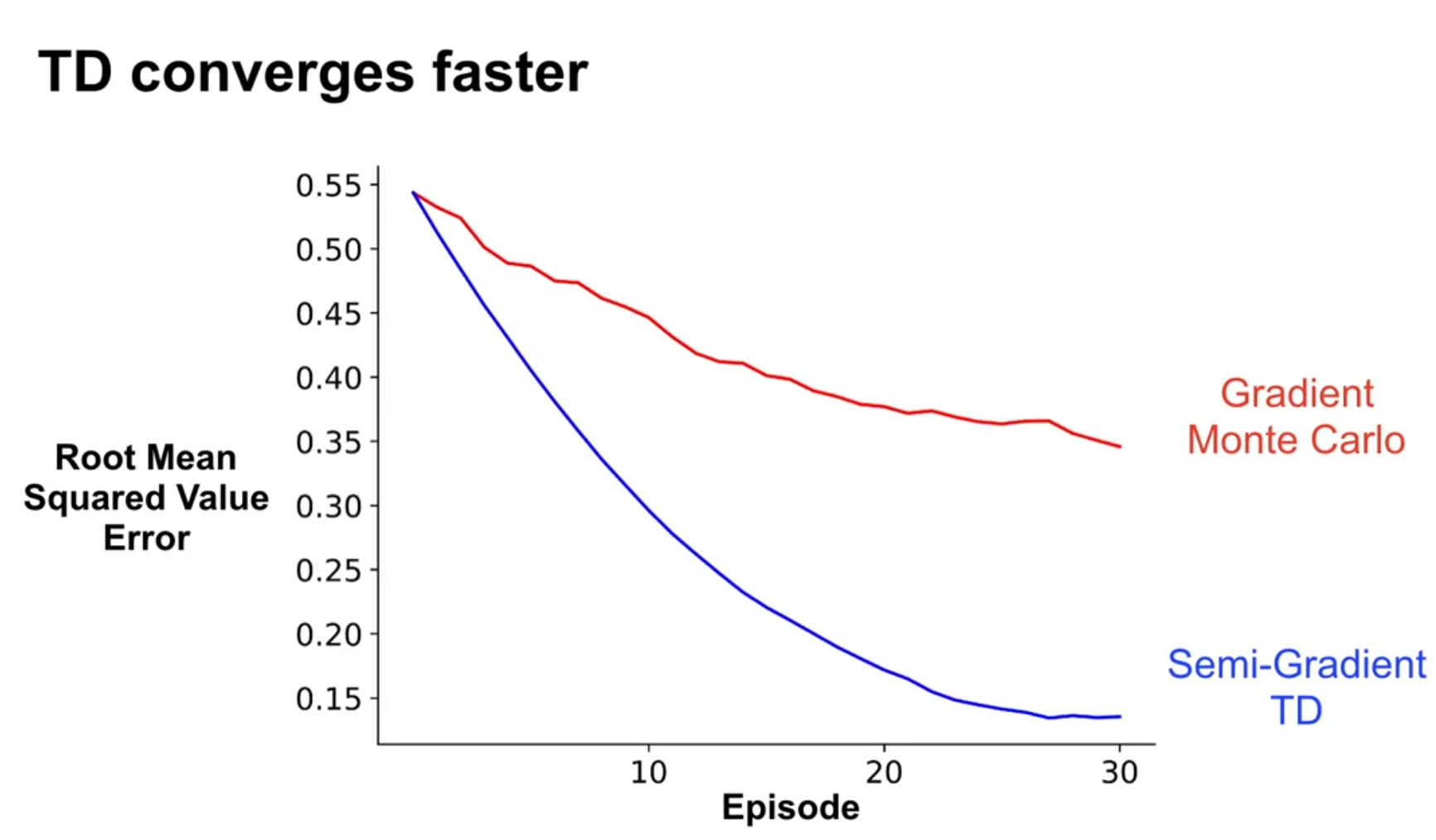
- We run the same random walk experiment for the 1000 episodes 1000 step random walk and we see that TD has a worse fit than MC on most of the range.
- We run a second experiments with only 30 episodes to see early learning performance and we see that TD has a better fit than MC on most of the range. In this case we used the best alpha for each method. MC needed a much smaller alpha to get a good fit.
- TD converges much faster than Gradient Monte Carlo because it updates the value function after every step.
- Gradient Monte Carlo can only update the value function after the episode is complete, which can be slow for long episodes.
- TD can learn online, while Gradient Monte Carlo can only learn offline.
- TD can learn from incomplete episodes, while Gradient Monte Carlo requires complete episodes.
- TD can learn from non-episodic tasks, while Gradient Monte Carlo can only learn from episodic tasks.
Doina Precup’s talk on Building Knowledge for AI Agents with Reinforcement Learning
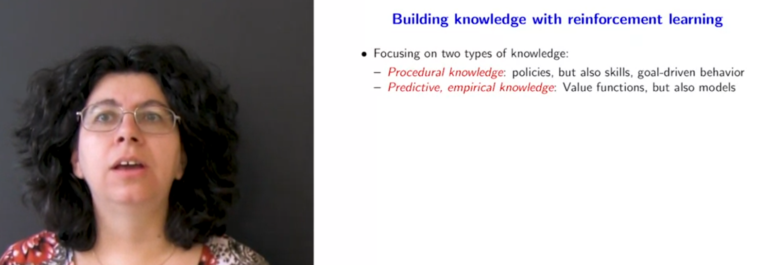
In this talk, Dorina Precup discusses the challenges of building knowledge for AI agents using reinforcement learning.
- Dorina Precup is a professor at McGill University and a research team lead at DeepMind.
- She is an expert in reinforcement learning and machine learning.
- Her interests are in the areas of abstractions.
- When I think about generalization in RL I think about:
- Learning a parameterized value function that can be used to estimate the value of any state.
- Learning a parameterized policy that can be used to select actions in any state.
- Being able to transfer this policy to a similar task
- Being able to learn using less interaction with the environment and more from replaying past experiences.
- Being able to learn from a small number of examples.
- Dorina talks about two other aspects of generalization:
- Action duration are one time step in an MDP, yet in reality some actions like traveling from one city to another require sticking to the action over an extended period of time.
- This might be happen through planning but idealy, agents should be able to learn skills which are sequences of actions that are executed over an extended period of time.
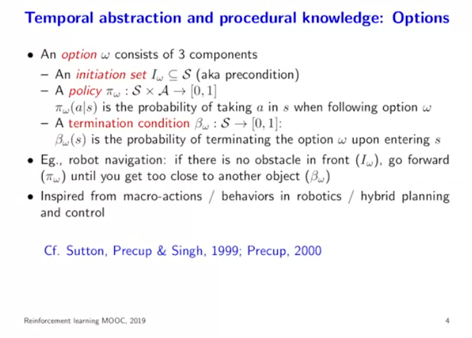
- This has been formalized in the literature as options.
- She references two sources
- (R. Sutton, Precup, and Singh 1999) a paper from 1999 on options in reinforcement learning.
- (Precup 2000) her doctoral thesis from 2000 on temporal abstraction in reinforcement learning.
- Options consists of
- an initiation set \iota_\omega(s) the precondition which is a probability of starting the option in state s.
- a policy \pi_\omega(a\mid s) that is executed in the option
- a termination condition \beta_\omega(s). the termination condition is a probability of terminating the option in state s.
- Options are “chunks of behavior” that can be executed over an extended period of time.
- The model will need to learn options and work with them.
- IT needs expected reward over the option.
- A transition model over the option.
- These models are predictive models about outcomes conditioned on the model being executed.
- Adding options to the model weakens the MDP assumption, because the option duration is not fixed so state now have a longer dependence is a sequence of actions that are not Markovian 2.
- Precup’s point out that combining temporal and spatial abstraction is an ongoing research challenge.
- She also points out that the model needs to learn the options and the value function at the same time.
- According to her profile Precup has a number of students working on this problem. Some additional references are:
- (Bacon, Harb, and Precup 2016) a paper from 2016 on option-critic architecture which extends actor-critic algorithms to work with options.
- Earlier work uses the term macro-actions to refer to options.
- (Bradtke and Duff 1994) a paper from 1994 on reinforcement learning with hierarchies of machines.
- This type of formulation seems very similar to that used by Judea Pearl in his structureal graphical model of Causality. If we can express options as a graph of states we can use his algorithms to infer the best options to take in a given state.
- options are like do operations (interventions)
- choosing between options is like conterfactual reasoning.
Lesson 4: Linear TD
Deriving the TD-update with linear function approximation
- Linear function is both:
- simple enough to be understood, yet
- powerful enough that with TD to be useful to create agents that are stornger than human Atari games.
- The TD-update with linear function approximation is a way to update the weights of the value function using the TD-error.
- The TD-update with linear function approximation works as follows:
- Compute the TD-error \delta as the difference between the one-step bootstrapped return and the approximate value of the next state.
- Update the weights \mathbf{w} in the direction of the TD-error.
recall the TD-update rule:
\delta \dot= R_{t+1} + \gamma \hat{v}(S_{t+1}, \mathbf{w}) - \hat{v}(S_t, \mathbf{w}) \\ w \leftarrow w + \alpha \delta_t \nabla \hat{v}(S_t, \mathbf{w}) in the linear case we can write the value function as:
\hat{v}(S_t, \mathbf{w}) \dot = \sum \mathbf{w}^T \mathbf{x}(S_t) \\ \nabla \hat{v}(S_t, \mathbf{w}) = \mathbf{x}(S_t)
w \leftarrow w + \alpha \delta_t \mathbf{x}(S_t)
Tabular TD(0) is a special case of linear semi-gradient TD(0)
- Tabular TD(0) is a special case of linear semi-gradient TD(0) where the features are one-hot encoded.
- In the tabular case, the weights are the same as the value function in the table.
- In the linear case, the weights are the parameters of the value function.
- Tabular TD(0) can be seen as a special case of linear semi-gradient TD(0) where the features are one-hot encoded.
Advantages of linear value function approximation over nonlinear
- Linear value function approximation has several advantages over nonlinear value function approximation:
- Linear value function approximation is computationally efficient and easy to implement.
- Linear value function approximation is easy to interpret and understand.
- Linear value function approximation is less prone to overfitting than nonlinear value function approximation.
- Linear value function approximation can be used to approximate any function, while nonlinear value function approximation is limited by the choice of features.
- If we have access to expert knowledge we can use it to define good features and use linear value function approximation to learn the value function quickly.
- Most of the theory of function approximation in reinforcement learning is based on linear value function approximation.
The fixed point of linear TD learning
w_{t+1} \dot= w_t + \alpha [R_{t+1} + \gamma \hat{v}(S_{t+1}, \mathbf{w}) - \hat{v}(S_t, \mathbf{w})] \nabla \hat{v}(S_t, \mathbf{w}) recall that in the linear case we defined the approximate value function as:
\hat{v}(S_{t+1}, \mathbf{w}) \cdot= \mathbf{w}^T \mathbf{x}(S_{t+1}) with :
- \mathbf{w} the weights of the value function
- \mathbf{x}(S_{t+1}) the features of the next state
using this definition we can write the update rule as:
\begin{align*} w_{t+1} & = w_t + \alpha [R_{t+1} + \gamma \mathbf{w}^T \mathbf{x}_{t+1} - \mathbf{w}^T \mathbf{x}] \mathbf{x}_t \newline &= w_t + \alpha [R_{t+1} \mathbf{x}_t - \mathbf{x}_t( \mathbf{x}_t - \gamma \mathbf{x_{t+1}})^T \mathbf{w_t}] \newline \end{align*}
let us now consider what this update looks like in expectation:
we can think about it as an expected update plus a noise term but the noise term is dominated by the behaviour of the expected update.
\mathbb{E}[\Delta w_{t}] = \alpha(b-Aw_t) where:
- b = \mathbb{E}[R_{t+1} \mathbf{x}_t] - expectation over the features and the rewards
- A = \mathbb{E}[\mathbf{x}_t( \mathbf{x}_t - \gamma \mathbf{x_{t+1}})^T] - an expectation over the rewards
note: this is a linear system of equations that looks like a linear regression problem.
when the weights do not change we have a fixed point:
\begin{align*} \mathbb{E}[\Delta w_{TD}] & = \alpha(b-Aw_{TD}) = 0 \newline \implies & w_{TD} = A^{-1}b \end{align*} \tag{11} more generally w_{TD} is the solution to this equation and we could show that it minimises
(b-Aw)^T(b-Aw) \tag{12}
this is related to Bellman equations via the projected Bellman error.
Theoretical guarantee on the mean squared value error at the TD fixed point
\overline{VE}(w_{TD}) \leq \frac{1}{1-\gamma} \min_{w} \overline{VE}(w) \tag{13}
- if \gamma \approx 1 then the mean squared value error at the TD fixed point can be large
- if \gamma \approx 0 then the mean squared value error at the TD fixed point can be small
- if the features representation is good then the two will be equal regardless of \gamma. since both will be almost zero.
Semi-gradient TD(0) algorithm
In the assignment I implemented the Semi-gradient TD(0) algorithm for value estimation.
References
Footnotes
Reuse
Citation
@online{bochman2024,
  author = {Bochman, Oren},
  title = {On-Policy {Prediction} with {Approximation}},
  date = {2024-04-01},
  url = {https://orenbochman.github.io/notes/RL/c3-w1.html},
  langid = {en}
}