Sample-based Learning Methods – Oren Bochman’s Blog

Lesson 1: What is a model?

Lesson Learning Goals

Describe what a model is and how they can be used #
Classify models as distribution models or sample models #
Identify when to use a distribution model or sample model #
Describe the advantages and disadvantages of sample models and distribution models #
Explain why sample models can be represented more compactly than distribution models #

What is a model and how can it be used?

A model is a simplified representation of the environment dynamics
Models can be used to simulate the environment
In this course a Model is a function that predicts the next state and reward given the current state and action
a transition model s_{t_+1} = f(s_t, a_t) predicts the next state given the current state and action
a reward model r_{t_+1} = f(s_t, a_t) predicts the reward given the current state and action

three other model types are mentioned in the ICML Tutorial on Model-Based Reinforcement Learning

Inverse models predict the action given the current state and next state a_{t+1} = f_s^{-1}(s_t, s_{t+1})
Distances models predict the distance between the current state and the goal state d_{ij} =d(s, s')
Future return models predict the future return given the current state and action G_t=Q(s_t, a_t) or G_t=V(s_t)

Why do we want to use models?

model allow us to simulate the environment without interacting with it.
this can increase sample efficiency - e.g. by replaying past experiences to propergate learning from goal to all predecessor states we have visited
this can reduce risks - e.g. by simulating dangerous situations instead of actually experiencing them.
this can reduce costs - e.g. by simulating costly actions in a simulated environment instead of paying the cost in the real environment.
this could be much faster than real-time interaction with the environment. Often in robotics simulation is orders of magnitude faster than real-time interaction.

Types of models

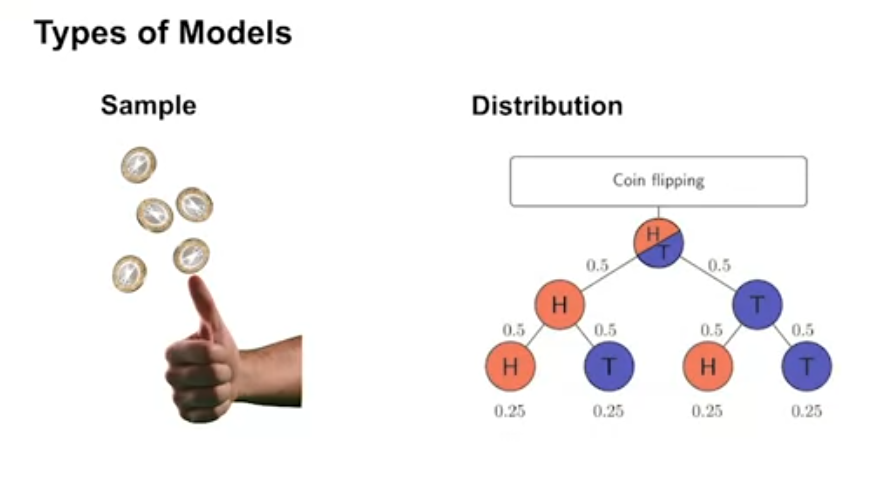
Distribution models predict the probability distribution of the next state and reward
Sample models predict a single next state and reward

Also there are:Environment simulator**

Chess Programs typicaly can simulate all possible movers and evaluate the board position (tacticaly and strategically). The difference between the current board position and the board position after a move is the reward.
(Silver et al. 2016) mentions an Environment simulator for the game of go
(Agostinelli et al. 2019) used a simulator of the rubik’s cube to train a reinforcement learning agent to solve the cube.
(Bellemare et al. 2012) used a simulator of the game of atari to train a reinforcement learning agent to play atari games.
(Todorov, Erez, and Tassa 2012) used a simulator of the physics of the real world to train a reinforcement learning agent to control a robot.
(Shen et al. 2018) used a simulator to train agents to navigate a graph using MCTS.
(Ellis et al. 2019) used a REPL environment to train a reinforcement learning agent to write code.

When to use a distribution model or sample model

Distribution models are useful when we need to know the probability of different outcomes
Sample models are useful when we need to simulate the environment

Advantages and disadvantages of sample models and distribution models

Sample models can be represented more compactly than distribution models
Distribution models can be more accurate than sample models
exact expectations can be computed from distribution models
assessing risks and uncertainties is easier with distribution models

Why sample models can be represented more compactly than distribution models

Sample models can be represented more compactly than distribution models because they only need to store a single next state and reward
Distribution models need to store the joint probability of each possible next state and reward pair
Sample models can be more efficient when we only need to simulate the environment

Lesson 2: Planning

Lesson Learning Goals

Explain how planning is used to improve policies #
Describe random-sample one-step tabular Q-planning #

How planning is used to improve policies

Planning is the process of using a model to improve a policy or value function
Planning can be used to improve a policy or value function without interacting with the environment
Planning can be used to improve a policy or value function more efficiently than direct RL updates

Random-sample one-step tabular Q-planning {#sec-l2g2}

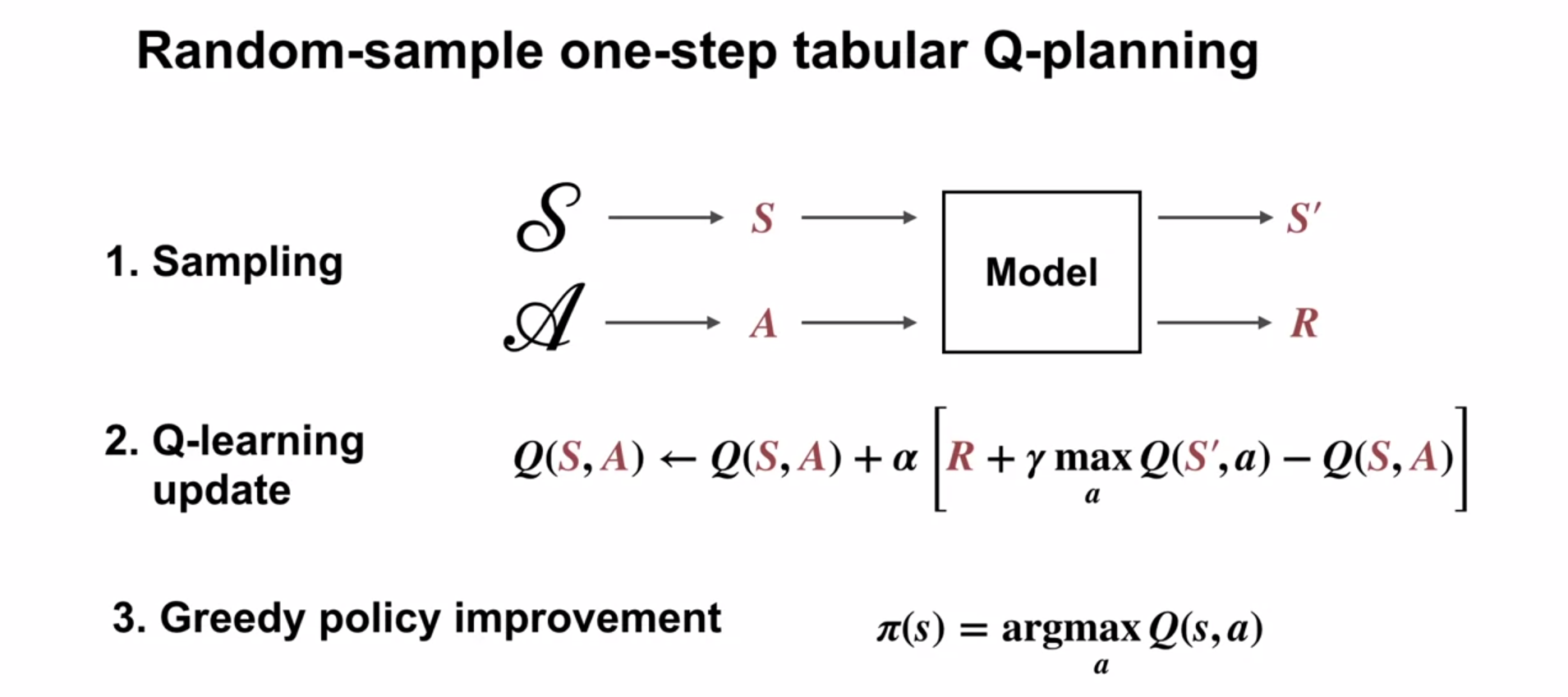
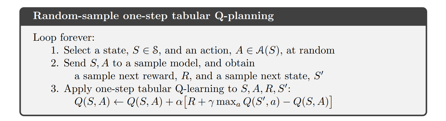
Tabular Q-planning is a planning algorithm that uses a sample model to improve a policy or value function
Tabular Q-planning uses a sample model to simulate the environment
Tabular Q-planning uses the simulated experience to improve a policy or value function

advantages of planning

Planning can be more efficient than direct RL updates
Planning can be used to improve a policy or value function without interacting with the environment
Planning can be used to improve a policy or value function more efficiently than direct RL updates

Lesson 3: Dyna as a formalism for planning

Lesson Learning Goals

Recognize that direct RL updates use experience from the environment to improve a policy or value function #
Recognize that planning updates use experience from a model to improve a policy or value function #
Describe how both direct RL and planning updates can be combined through the Dyna architecture #
Describe the Tabular Dyna-Q algorithm #
Identify the direct-RL and planning updates in Tabular Dyna-Q #
Identify the model learning and search control components of Tabular Dyna-Q #
Describe how learning from both direct and simulated experience impacts performance #
Describe how simulated experience can be useful when the model is accurate #

Direct RL updates use experience from the environment to improve a policy or value function

Direct RL updates use experience from the environment to improve a policy or value function
Direct RL updates can be used to improve a policy or value function by interacting with the environment

Planning updates use experience from a model to improve a policy or value function

Planning updates use experience from a model to improve a policy or value function
Planning updates can be used to improve a policy or value function without interacting with the environment

Both direct RL and planning updates can be combined through the Dyna architecture

Dyna architecture combines direct RL updates and planning updates to improve a policy or value function
Dyna architecture uses a model to simulate the environment
Dyna architecture uses the simulated experience to improve a policy or value function

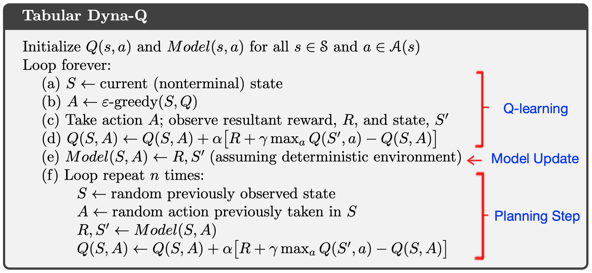
The Tabular Dyna-Q algorithm

Tabular Dyna-Q is a planning algorithm that uses a sample model to improve a policy or value function
Tabular Dyna-Q uses a sample model to simulate the environment
Tabular Dyna-Q uses the simulated experience to improve a policy or value function

Exercise 8.2 Why did the Dyna agent with exploration bonus, Dyna-Q+, perform better in the first phase as well as in the second phase of the blocking and shortcut experiments?

Dyna-Q+ is like a generalized UCB while Dyna-Q+ is like a generalized epsilon greedy alg. Dyna-Q+ is doing more efficent exploration. It will revisits will be more spread out more over time but it scheme also tends to increases in non independent way - probabilities for unvisited regions keep growing so if it starts exploring it may like doing an extended sequence till it gets to a dead end.
Dyna Q exploration is independent for each state,action combo so retrying sequences get asymptotically less likely with time.

Exercise 8.3 Careful inspection of Figure 8.5 reveals that the difference between Dyna-Q+ and Dyna-Q narrowed slightly over the first part of the experiment. What is the reason for this?

Dyna-Q+ is more efficient at exploring so it learned a better policy, but since the environment was static Dyna-Q got to catch up, but it never reached the same policy.

Exercise 8.5 How might the tabular Dyna-Q algorithm shown on page 164 be modified to handle stochastic environments? How might this modification perform poorly on changing environments such as considered in this section? How could the algorithm be modified to handle stochastic environments and changing environments?

to hadle a stochastic environment one would need to to model probabilities of stochastic dynamics. One way to do this is to use Bayesian updating with a dericlet prior and a multinomial posterior.
This modification would likely fare much worse since learning low probability transitions would require many visits to discover.
In the case of changing environment it would also take much longer for new state to be reflected in the model (if a state was visited 10 with just one transition and then the transition changed to another state then it would take many more than 10 vistis to quash the old probability and get the new one correct to 10%
This means that we adding a forgetting rule might be better then the plain derichlet-multinomial model.
To handle both stochastic and changing updates we may want to
1. track the recency of the last visit and reward this option like in dyna-q plus.
2. decay old probabilities - would require storing the time for each visit - i.e. path dependent model.
3. A better idea is to use a hirachial model with parial pooling representing short term and long term transitions - this could fix the problem of decay by simply giving greater weight to the smaller more recent model.
The short term would track the last k visits in each state and the long term all the visits. We could then do partial pooling between these two estimators with much greater emphasis on the recent one!

Direct-RL and planning updates in Tabular Dyna-Q

Tabular Dyna-Q uses direct RL updates to improve a policy or value function
Tabular Dyna-Q uses planning updates to improve a policy or value function

Model learning and search control components of Tabular Dyna-Q

Tabular Dyna-Q uses a sample model to simulate the environment
Tabular Dyna-Q uses the simulated experience to improve a policy or value function

Learning from both direct and simulated experience impacts performance

Learning from both direct and simulated experience can improve performance
Learning from both direct and simulated experience can be more efficient than direct RL updates

Simulated experience can be useful when the model is accurate

Simulated experience can be useful when the model is accurate
Simulated experience can be used to improve a policy or value function without interacting with the environment

Lesson 4: Dealing with inaccurate models

Lesson Learning Goals

Identify ways in which models can be inaccurate #
Explain the effects of planning with an inaccurate model #
Describe how Dyna can plan successfully with a partially inaccurate model #
Explain how model inaccuracies produce another exploration-exploitation trade-off #
Describe how Dyna-Q+ proposes a way to address this trade-off #

Ways in which models can be inaccurate

Models can be inaccurate for many reasons
because they have not sampled all actions in all states
because the environment is has changed since the model was learned
if the environment is stochastic

Effects of planning with an inaccurate model

Planning with an inaccurate model can cause the value function to become worse
Planning with an inaccurate model can lead to sub-optimal policies

Dyna can plan successfully with a partially inaccurate model

Dyna can plan successfully with a partially inaccurate model
Dyna can use direct RL updates to improve a policy or value function as well as the model
Dyna can use planning updates to improve a policy or value function

Model inaccuracies produce another exploration-exploitation trade-off

Model inaccuracies produce another exploration-exploitation trade-off
exploit an inaccurate model to improve the policy
revisit states/actions with low value to update the model
Can we use an inverse sort of planning to identify states for which the model is inaccurate?
Model inaccuracies can lead to suboptimal policies
Model inaccuracies can lead to poor performance

Dyna-Q+ proposes a way to address this trade-off

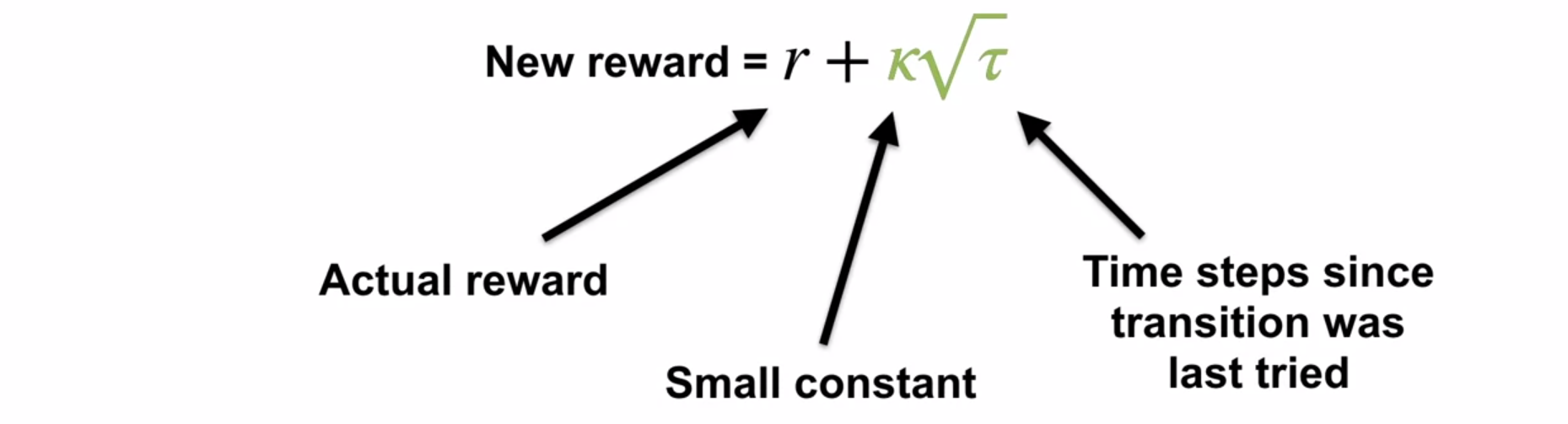
Dyna-Q+ proposes a way to address this trade-off
Dyna-Q+ uses a bonus reward to encourage exploration
Dyna-Q+ can improve performance when the model is inaccurate

Drew Bagnell on self-driving cars robotics and model-based reinforcement learning

Drew Bagnell is a professor at Carnegie Mellon University and the CTO at Aurora innovation.

He has worked on self-driving cars and robotics. He has also worked on model-based reinforcement learning. He point out a dirty little secret that model-based reinforcement learning is a key technology for robotics.

He points out that the real world is expensive and dangerous. Using model based reinforcement learning can reduce the number of interactions with the real world and along learning about risky actions in the simulated world to improve performance in the real world. Also as we pointer out before this can usually be done much faster than real-time interaction with the environment.

Sample complexity: how many real-world samples are required to achieve high performance? It takes exponentially fewer interactions with a model than without. Not really sure what exponentially fewer means here - but it’s a lot fewer.

Quadratic value function approximation goes back to optimal control in the 1960s. It’s continuous in states and actions. This is a method that should be part of the next course but isn’t covered there either

For linear transition dynamics with quadratic costs/rewards, it’s exact. For local convex / concave points, it is a good approximation of the true action-value function.

Here is the math from his slide:

Quadratic value function approximation

Q_t(x,a) = \begin{bmatrix} x \\ a \\ \end{bmatrix}^T \begin{bmatrix} Q_{xx} && Q_{xa} \\ Q_{xa} && Q_{uu} \\ \end{bmatrix} \begin{bmatrix} x \\ a \\ \end{bmatrix}^T + \begin{bmatrix} q_x \\ q_a \\ \end{bmatrix}^T \begin{bmatrix} x \\ a \\ \end{bmatrix} + const \tag{1}

The approximation allows for calculating the optimal action-value in closed form (finite number of standard operations) even with continuous actions.

Differential dynamic programming takes advantage of the technique above.

So this seems complicated - because of matrix maths. But intuitively this is something we like to do in physics - add the term for the second derivative
in the taylor series approximation of our function.

The 2nd paper is particularly clear and easy to work through for the approach just described.

timeline

    title Bandit Algorithms Timeline

    
        1952 : Thompson Sampling
        1955 : Upper Confidence Bound (UCB)
        1963 : Epsilon-Greedy
        2002 : Bayesian UCB
        2011 : Bayesian Bandits
        2012 : Contextual Bandits

%%{init: {'theme': 'base', 'themeVariables': { 'timeline': { 'nodeSpacing': 50, 'sectionSpacing': 100, 'verticalStartPosition': 50, 'verticalSectionStartPosition': 50 }}}}%%
timeline
    direction TD
    title Reinforcement Learning Algorithms Timeline


    
        1948 : Monte Carlo Methods
        1950 : Bellman Optimality Equations
        1957 : Dynamic Programming
        1959 : Temporal Difference Learning (TD)
        1960 : Policy Iteration
        1963 : Value Iteration
        1983 : Q-Learning
        1984 : Expected SARSA
        1990 : Dyna-Q : Dyna-Q+
        1992 : SARSA
        1994 : Monte Carlo with E-Soft
        1995 : Monte Carlo with Exploring Starts
             : Generalized Policy Iteration (GPI)
        1998 : Semi-Gradient TD
        2000 : Differential Semi-Gradient SARSA
        2001 : Gradient Monte Carlo (Gradient MC)
        2003 : Gaussian Actor-Critic
             : Softmax Actor-Critic
             : Deep Q-Network (DQN)

References

Materials from ICML Tutorial on Model-Based Reinforcement Learning:

the page above contains the following materials as well as an extensive bibliography.

From Bagnell’s talk:

References

Agostinelli, Forest, S. McAleer, A. Shmakov, and P. Baldi. 2019. “Solving the Rubik’s Cube with Deep Reinforcement Learning and Search.” Nature Machine Intelligence 1: 356–63.

Bellemare, Marc G., Yavar Naddaf, J. Veness, and Michael Bowling. 2012. “The Arcade Learning Environment: An Evaluation Platform for General Agents.” ArXiv abs/1207.4708.

Ellis, Kevin, Maxwell Nye, Yewen Pu, Felix Sosa, J. Tenenbaum, and Armando Solar-Lezama. 2019. “Write, Execute, Assess: Program Synthesis with a REPL,” 9165–74.

Shen, Yelong, Jianshu Chen, Po-Sen Huang, Yuqing Guo, and Jianfeng Gao. 2018. “M-Walk: Learning to Walk in Graph with Monte Carlo Tree Search.” In Neural Information Processing Systems.

Silver, David, Aja Huang, Chris J. Maddison, A. Guez, L. Sifre, George van den Driessche, Julian Schrittwieser, et al. 2016. “Mastering the Game of Go with Deep Neural Networks and Tree Search.” Nature 529: 484–89.

Todorov, E., Tom Erez, and Yuval Tassa. 2012. “MuJoCo: A Physics Engine for Model-Based Control.” 2012 IEEE/RSJ International Conference on Intelligent Robots and Systems, 5026–33.

Reuse

CC SA BY-NC-ND

Citation

BibTeX citation:

@online{bochman2024,
  author = {Bochman, Oren},
  title = {Sample-Based {Learning} {Methods}},
  date = {2024-03-04},
  url = {https://orenbochman.github.io/notes/RL/c2-w4.html},
  langid = {en}
}

For attribution, please cite this work as:

Bochman, Oren. 2024. “Sample-Based Learning Methods.” March 4, 2024. https://orenbochman.github.io/notes/RL/c2-w4.html.