Lesson 1: The K-Armed Bandit

Read

Goals

Understand the temporal nature of the bandit problem #
Define k-armed bandit problem #
Define action-values and the greedy action selection method #
Define reward, time steps, and value functions #

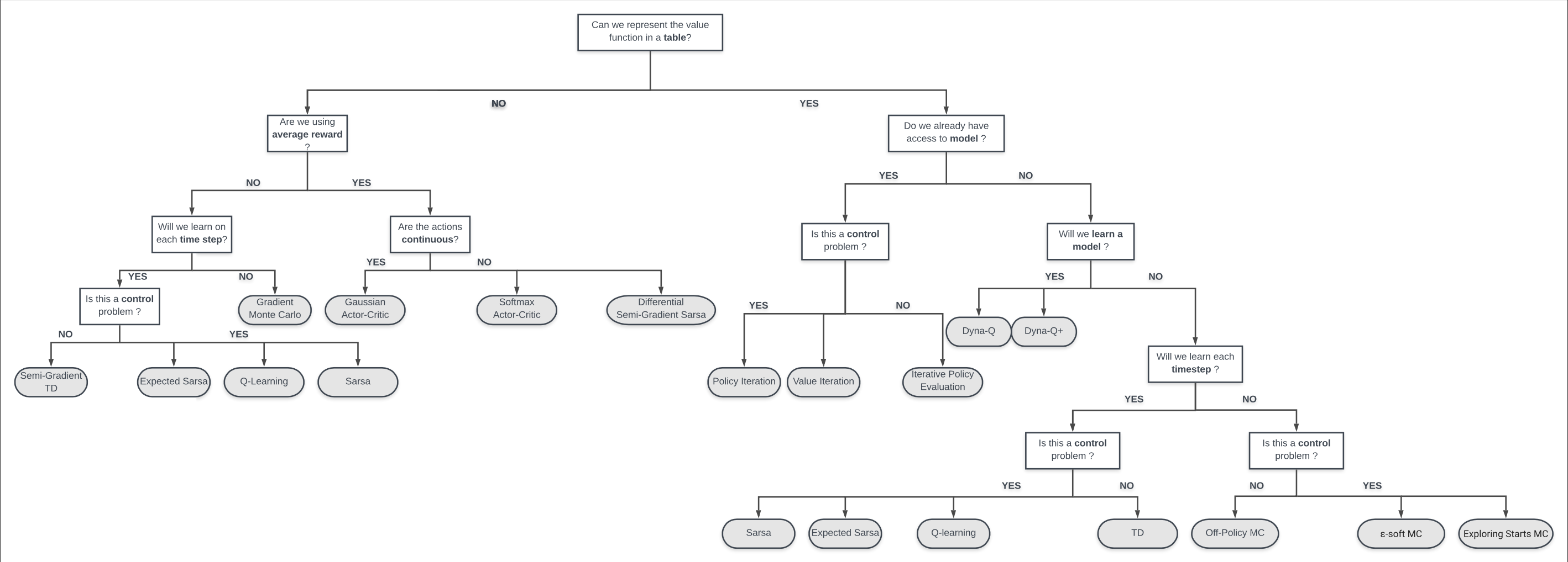
In reinforcement learning, the agent generates its own training data by interacting with the world. The agent must learn the consequences of his own actions through trial and error, rather than being told the correct action – (Matha White 2020)

K-armed bandits 🐙

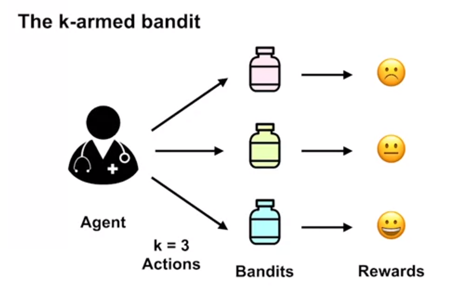
In the k-armed bandit problem there is an agent who is assigned a state s by the environment and must learn which action a from the possible set of actions A leads to the goal state through a signal based on the greatest expected reward.

One way this can be achieved is using a Bayesian updating scheme starting from a uniform prior.

Temporal nature of the bandit problem

The bandit problem cam be static problem with a fixed reward distribution. However, more generally it is a temporal problem when the rewards distribution changes over time and agent must learn to adapt to these changes.

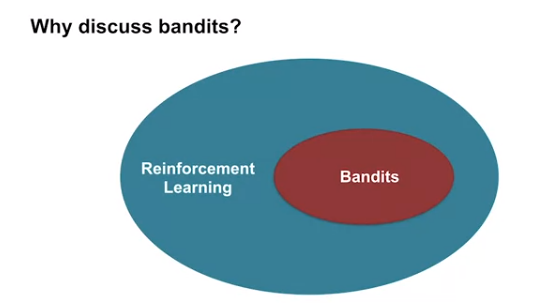
Difference between bandits and RL

In the typical bandit setting there is only one state. So after we pull the arm nothing in the problem changes.

Bandits problems where agents can discriminate between states are called contextual bandits.

However, bandits embody one of the main themes of RL - that of estimating an expected reward for different actions.

In the more general RL setting we will be interested in more general problems where actions will lead the agent to new states and the goal is some specific state we need to reach.

bandit

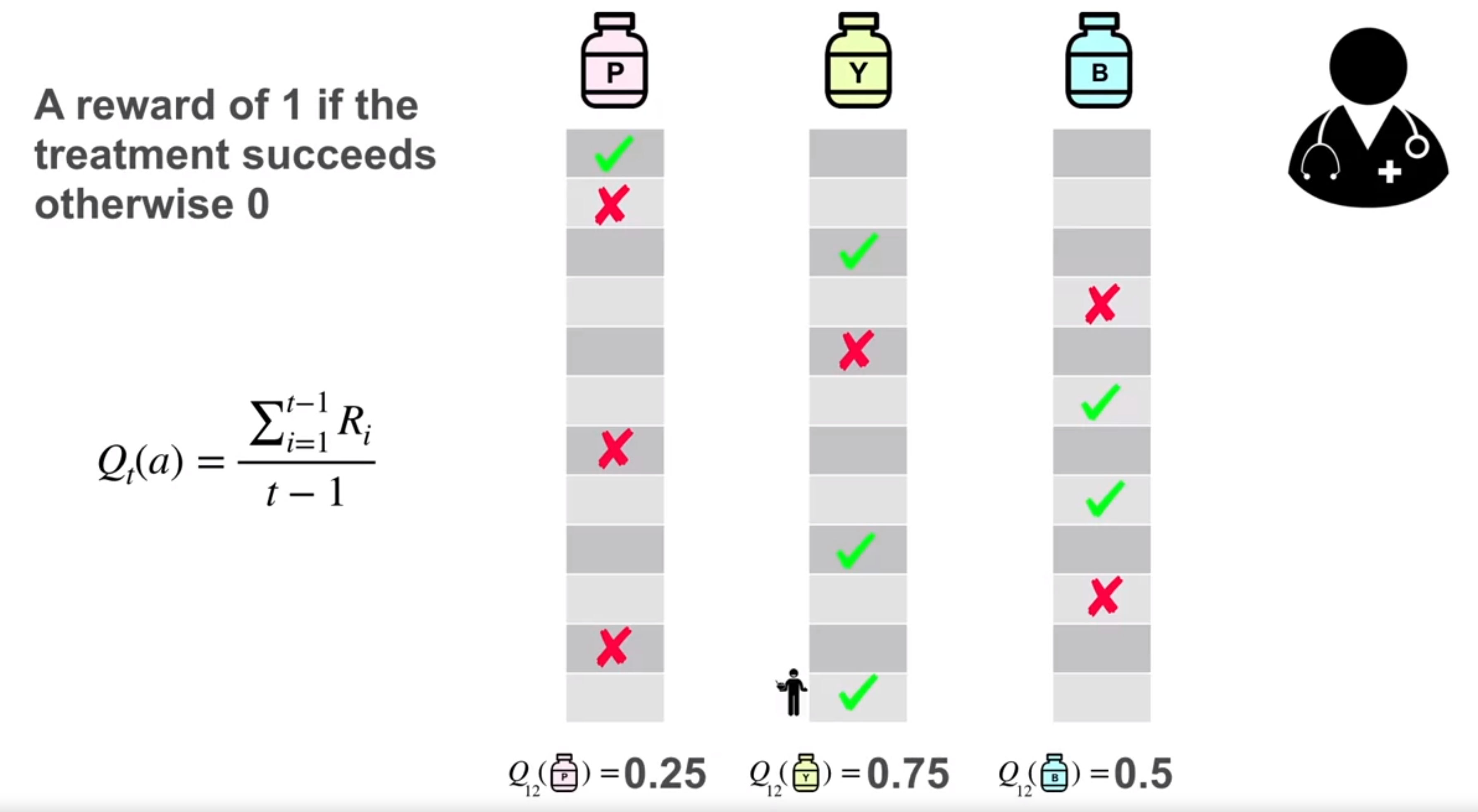
Example 1 (Using Multi-armed bandit to randomize a medical trial)

agent is the doctor
actions {blue, yellow, red} treatment
k = 3
the rewards are the health of the patients’ blood pressure.
a random trial in which a doctor need to pick one of three treatments.
q(a) is the mean of the blood pressure for the patient.

Action Values and Greedy Action Selection

The value of an action is its expected reward which can be expressed mathematically as:

\begin{align} q_{\star}(a) & \doteq \mathbb{E}[R_t \vert A_t=a] \space \forall a \in \{a_1 ... a_k\} \newline & = \sum_r p(r|a)r \qquad \text{(action value)} \end{align} \tag{1}

where:

\doteq means definition
\mathbb{E}[r \vert a] means expectation of a reward given some action a Since agents want to maximize rewards, recalling the definition of expectations we can write this as:

The goal of the agent is to maximize the expected reward which we can express mathematically as:

\arg\max_a q(a)=\sum_r p(r \vert a) \times r \qquad \text{(Greedification)} \tag{2}

where:

\arg \max_a means the argument a maximizes - so the agent is looking for the action that maximizes the expected reward and the outcome is an action.

Reward, Return, and Value Functions

The reward r is the immediate feedback from the environment after the agent takes an action.

The return G_t is the total discounted reward from time-step t.

The value function v(s) of an MRP is the expected return starting from state s.

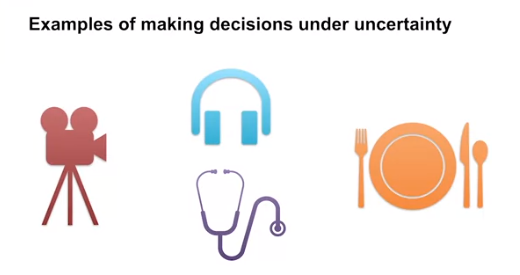
example of decisions under uncertainty:

movie recommendation.
clinical trials.
music recommendation.
food ordering at a restaurant.

It best to consider issues and algorithms design choices in the simplest setting first. The bandit problem is the simplest setting for RL. More advanced algorithms will incorporate parts we use to solve this simple settings.

maximizing rewards.
balancing exploration and exploitation.
estimating expected rewards for different actions.

are all problems we will encounter in both the bandit and the more general RL setting.

Lesson 2: What to learn: understanding Action Values

Goals

Define action-value estimation methods. #
Define exploration and exploitation #
Select actions greedily using an action-value function #
Define online learning #
Understand a simple online sample-average action-value estimation method #
Define the general online update equation #

What are action-value estimation methods?

In Tabular RL settings The action value function q is nothing more than a table with one {state, action} pair per row and its value. More generally, like when we will consider function approximation in course 3, it is a mapping from {state, action} pair to a expected reward.

State s	Action a	Action value q(s,a)
0	red treatment	0.25
0	yellow treatment	0.75
0	blue treatment	0.5

The higher the action value q(a) of an action a, the more likely it is to lead us to a better state which is closer to the objective. We can choose for each state the best or one of the best choices giving us a plan for navigating the state space to the goal state.

Q_t(a) \doteq \frac{\text{sum of rewards for action a taken time } t}{\text{number of times action a was taken prior to } t} = \frac{\sum_{i=1}^{t-1} R_i}{t-1} \qquad \tag{3}

The main idea of RL is that we can propagate values from an one adjacent state to another. We can start with the uniform stochastic policy and use it to estimate/learn the action values. Action values will decrease for actions leads to a dead end. And it will increase in the direction of the goal but only once the influence of the goal has propagated. A continuing theme in RL is trying to increase the efficiency for propagation of rewards across the action values.

Knowing the minimum number of action needed to reach a goal can be an approximate indicator of the action value.

A second idea is that once we have let the influence of dead end and the goals spread enough we may have enough information to improve the initial action value to a point where each action is the one of the best choices. We call picking the one of the best action greedy selection and it leads to a deterministic policy. This is the optimal policy, it might not be unique since some actions might be tied in terms of their rewards. However for all of these we cannot do any better.

Exploration and Exploitation definition and dilemma

In the bandit setting we can define:

Exploration: Testing any action that might be better than our best.
Exploitation: Using the best action.

Should the doctor explore new treatments that might harm his patients or exploit the current treatment. In real life bacteria gain immunity to antibiotics so there is merit to exploring new treatments. However, a new treatment can be harmful to some patients. Ideally we want to enjoy the benefits of the best treatment but to be open to new and better alternatives but we can only do one at a time.

Since exploitation is by definition mutually exclusive with exploration we must choose one and give up the benefits of the other. This is the dilemma of Exploration and Exploitation. How an agent resolves this dilemma in practice depends on the agent’s preferences and the type of state space it inhabits, if it has just started or encounters a changing landscape, it should make an effort to explore, on the other hand if it has explored enough to be certain of a global maximum it would prefer to exploit.

Defining Online learning ?

Online learning: learning by updating the agent’s value function or the action value function step by step as an agent transverses the states seeking the goal. Online learning is important to handle MDP which can change.

One simple way an agent can use online learning is to try actions by random and keep track of the subsequent states. Eventually we should reach the goal state. If we repeat this many times we can estimate the expected rewards for each action.

Sample Average Method for estimating Action Values Incrementally

Action values help us make decision. Let’s try and make estimate action values more formal using the following method:

q_t(a)=\frac{\text{sum or rewards when a taken prior to t}}{\text{number of times a taken prior to t}} =\frac{\sum_{t=1}^{t-1} R_i \mathbb{I}_{A_i=a}}{\sum_{t=1}^{t-1}\mathbb{I}_{A_i=a} } \qquad

\begin{align} Q_{n+1} &= \frac{1}{n} \sum_{i=1}^n R_i \newline & = \frac{1}{n} \Bigg(R_n + \sum_i^{n-1} R_i\Bigg) \newline & = \frac{1}{n} \Bigg(R_n + (n-1) \frac{1}{(n-1)}\sum_i^{n-1} R_i\Bigg) \newline &= \frac{1}{n} \Big(R_n + (n-1) Q_{n}\Big) \newline &= \frac{1}{n} \Big(R_n + nQ_{n} -Q_{n} \Big) \newline &= Q_n + \frac{1}{n} \Big[R_n - Q_{n}\Big] \end{align} \tag{4}

What are action-value estimation methods?

We can now state this in English as:

\text{New Estimate} \leftarrow \text{Old Estimate} + \text{Step Size } \times [\text{Target} - \text{Old Estimate}] \qquad

here:

step size can be adaptive - changing over time. but typically it is constant and in the range (0,1) to avoid divergence.
for the sample average method the step size is \frac{1}{n} where n is the number of times the action has been taken.
(Target - OldEstimate) is called the error.

More generally we will use the update rule as:

Q_{n+1} = Q_n + \alpha \Big[R_n - Q_{n}\Big] \qquad a\in (0,1) \tag{5}

\begin{algorithm} \caption{Simple Bandit($\epsilon$)}\begin{algorithmic} \State $Q(a) \leftarrow 0\ \forall a\ $ \Comment{ $\textcolor{blue}{initialize\ action\ values}$} \State $N(a) \leftarrow 0\ \forall a\ $ \Comment{ $\textcolor{blue}{initialize\ counter\ for\ actions\ taken}$} \For{$t = 1, 2, \ldots \infty$} \State $A_t \leftarrow \begin{cases} \arg\max_a Q(a) & \text{with probability } 1 - \epsilon \\ \text{a random action} & \text{with probability } \epsilon \end{cases}$ \State $R_t \leftarrow \text{Bandit}(A_t)$ \State $N(A_t) \leftarrow N(A_t) + 1$ \State $Q(A_t) \leftarrow Q(A_t) + \frac{1}{N(A_t)}[R_t - Q(A_t)]$ \EndFor \end{algorithmic} \end{algorithm}

Lesson 3: Exploration vs Exploitation

Goals

Define \epsilon-greedy #
Compare the short-term benefits of exploitation and the long-term benefits of exploration #
Understand optimistic initial values #
Describe the benefits of optimistic initial values for early exploration #
Explain the criticisms of optimistic initial values #
Describe the upper confidence bound action selection method #
Define optimism in the face of uncertainty #

the following is a Bernoulli greedy algorithm

\begin{algorithm} \caption{BernGreedy(K, α, β)}\begin{algorithmic} \For{$t = 1, 2, . . .$} \State \State \Comment{ estimate model} \For{$k = 1, . . . , K$} \State $\hat\theta_k \leftarrow a_k / (α_k + β_k)$ \EndFor \State \Comment{ select and apply action:} \State $x_t \leftarrow \arg\max_k \hat{\theta}_k$ \State Apply $x_t$ and observe $r_t$ \State \Comment{ update distribution:} \State $(α_{x_t}, β_{x_t}) \leftarrow (α_{x_t} + r_t, β_{x_t} + 1 − r_t)$ \EndFor \end{algorithmic} \end{algorithm}

Ɛ-Greedy Policies

The Ɛ-greedy policy uses a simple heuristic to balance exploration with exploitation. The idea is to choose the best action with probability 1-\epsilon and to choose a random action with probability \epsilon.

\begin{algorithm} \caption{EpsilonGreedy(K, α, β)}\begin{algorithmic} \For{$t = 1, 2, \ldots $} \State p = random() \If {$p < \epsilon$} \State select radom action $x_t \qquad$ \Comment{explore} \Else \State select $x_t = \arg\max_k \hat{\theta}_k \qquad$ \Comment{exploit} \EndIf \EndFor \end{algorithmic} \end{algorithm}

The problem with Ɛ-greedy policies

A problem with Ɛ-greedy is that it is not optimal in the long run.
Even after it has found the best course of action it will continue to explore with probability \epsilon.
This is because the policy is not adaptive.
One method is too reduce \epsilon over time. However unless there is a feedback from the environment this will likely stop exploring too soon or too late thus providing sub-optimal returns.

The following is a simple implementation of the Ɛ-greedy algorithm in Python from geeksforgeeks.org

# Import required libraries 
import numpy as np 
import matplotlib.pyplot as plt 
  
# Define Action class 
class Actions: 
  def __init__(self, m): 
    self.m = m 
    self.mean = 0
    self.N = 0
  
  # Choose a random action 
  def choose(self):  
    return np.random.randn() + self.m 
  
  # Update the action-value estimate 
  def update(self, x): 
    self.N += 1
    self.mean = (1 - 1.0 / self.N)*self.mean + 1.0 / self.N * x 
  
  
def run_experiment(m1, m2, m3, eps, N): 
      
  actions = [Actions(m1), Actions(m2), Actions(m3)] 
  
  data = np.empty(N) 
    
  for i in range(N): 
    # epsilon greedy 
    p = np.random.random() 
    if p < eps: 
      j = np.random.choice(3) 
    else: 
      j = np.argmax([a.mean for a in actions]) 
    x = actions[j].choose() 
    actions[j].update(x) 
  
    # for the plot 
    data[i] = x 
  cumulative_average = np.cumsum(data) / (np.arange(N) + 1) 
  
  # plot moving average ctr 
  plt.plot(cumulative_average) 
  plt.plot(np.ones(N)*m1) 
  plt.plot(np.ones(N)*m2) 
  plt.plot(np.ones(N)*m3) 
  plt.xscale('log') 
  plt.show() 
  
  for a in actions: 
    print(a.mean) 
  
  return cumulative_average

c_1 = run_experiment(1.0, 2.0, 3.0, 0.1, 100000) 
#print(c_1)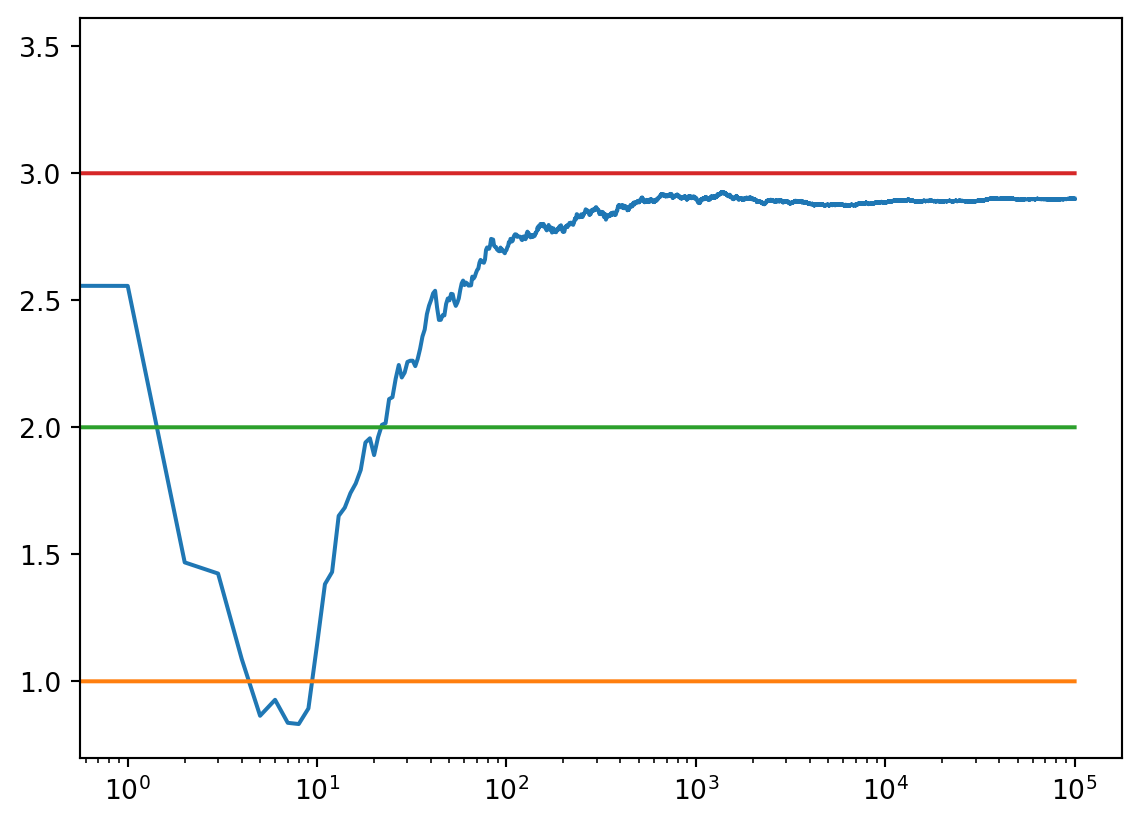

1.0094780662240135
2.0245712811610135
2.9972000253754496

c_05 = run_experiment(1.0, 2.0, 3.0, 0.05, 100000) 
#print(c_05)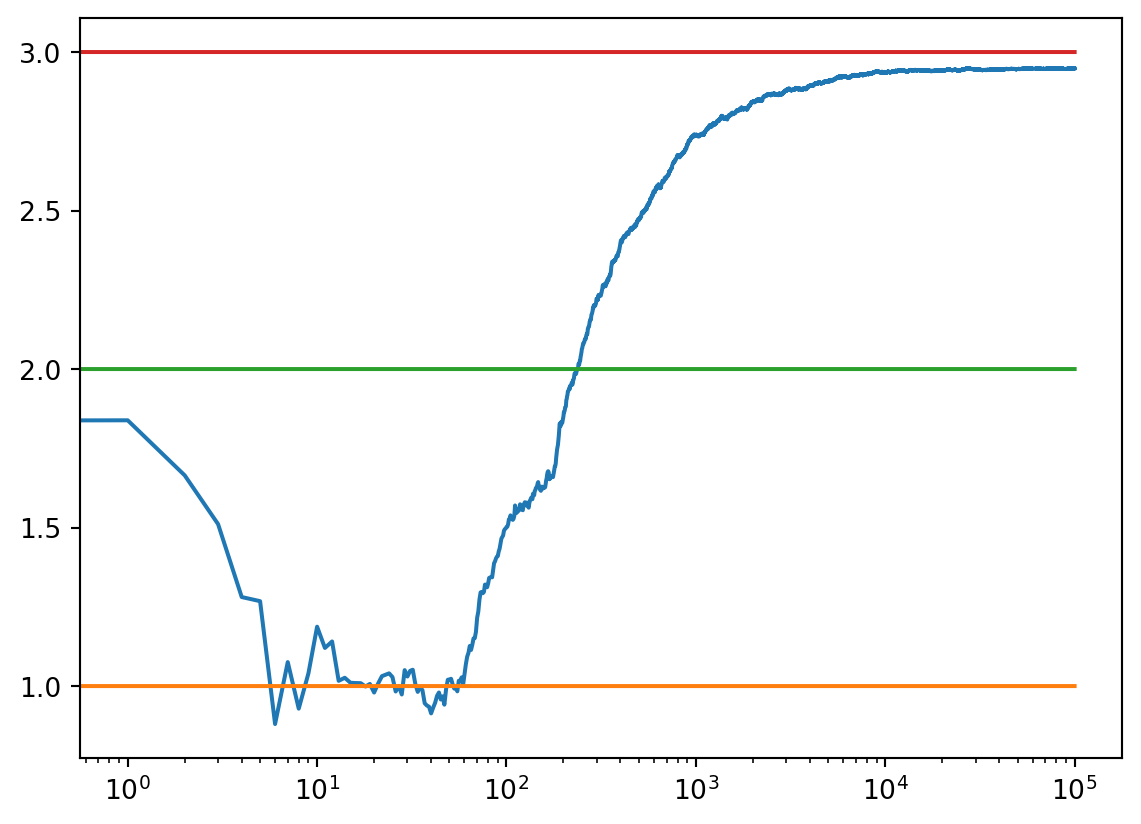

1.0017659185071361
1.961083641939731
3.0005090154235132

c_01 = run_experiment(1.0, 2.0, 3.0, 0.01, 100000) 
#print(c_01)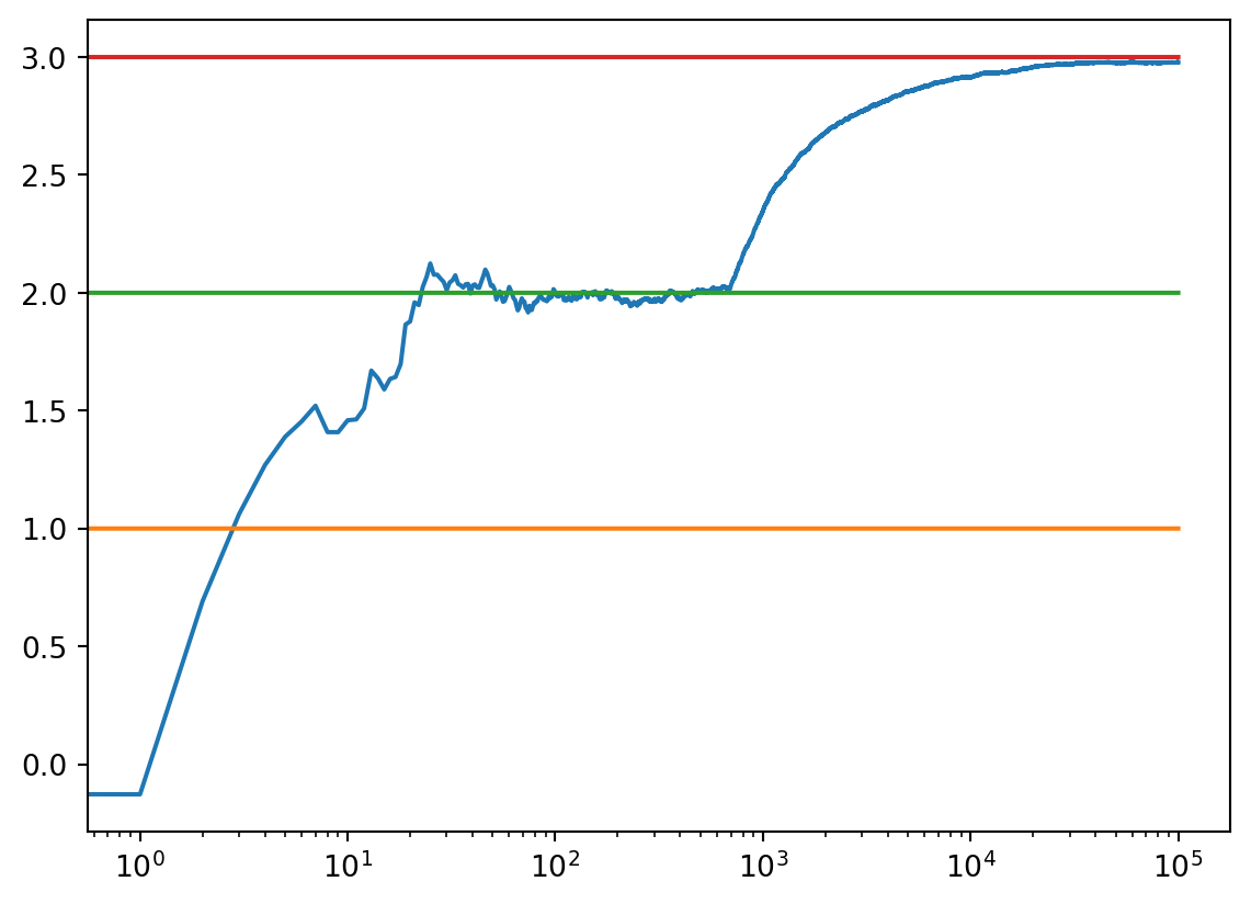

1.0146717998407884
1.9924957557231526
2.9996614535157367

# log scale plot 
plt.plot(c_1, label ='eps = 0.1') 
plt.plot(c_05, label ='eps = 0.05') 
plt.plot(c_01, label ='eps = 0.01') 
plt.legend() 
plt.xscale('log') 
plt.show()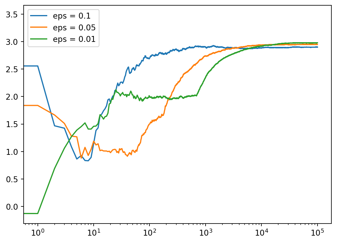

Benefits of Exploitation & Exploration

In the short term we may maximize rewards following the best known course of action. However this may represent a local maximum.
In the long term agents that explore different options and keep uncovering better options until they find the best course of action corresponding to the global maximum.

To get the best of both worlds we need to balance exploration and exploitation ideally using a policy that uses feedback to adapt to its environment.

Optimistic initial values

Optimistic initial values: Setting all initially action values greater than the algorithmically available values in [0,1]

The methods we have discussed are dependent on the initial action-value estimates, Q_1(a). In the language of statistics, we call these methods biased by their initial estimates. For the sample-average methods, the bias disappears once all actions have been selected at least once. For methods with constant \alpha, the bias is permanent, though decreasing over time.

\begin{algorithm} \caption{OptimisticBernGreedy(K, α, β)}\begin{algorithmic} \For{$t = 1, 2, . . .$} \State \State \Comment{ estimate model} \For{$k = 1, . . . , K$} \State $\hat\theta_k \leftarrow 1 \qquad$ \Comment{optimistic initial value} \EndFor \State \Comment{ select and apply action:} \State $x_t \leftarrow \arg\max_k \hat{\theta}_k$ \State Apply $x_t$ and observe $r_t$ \State \Comment{ update distribution:} \State $(α_{x_t}, β_{x_t}) \leftarrow (α_{x_t} + r_t, β_{x_t} + 1 − r_t)$ \EndFor \end{algorithmic} \end{algorithm}

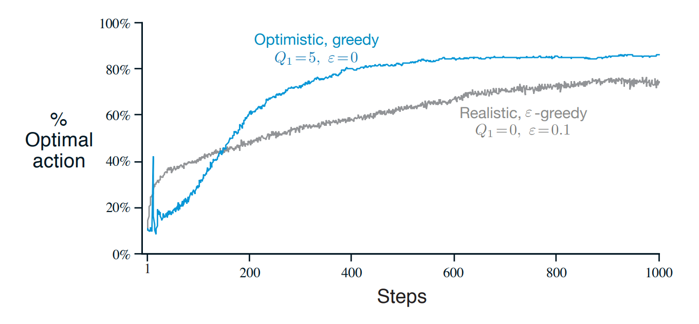
Benefits of optimistic initial values for early exploration

Setting the initial action values to be higher than the true values has the effect of causing various bandit algorithm to try to exploit them - only to find out that most values are not as rewarding as it was led to expect.

What happens is that the algorithm will initially explore more than it would have otherwise. Possibly even trying all the actions at least once.

In the short-term it will perform worse than Ɛ- greedy which tend to exploit. But as more of the state space is explored at least once the algorithm will beat an Ɛ-greedy policy which can take far longer to explore the space and find the optimal options.

The effect of optimistic initial action-value estimates

Criticisms of optimistic initial values

Optimistic initial values only drive early exploration. The agent will stop exploring once this is done.
For a non-stationary problems - this is inadequate.
In a real world problems the maximum reward is an unknown quantity.

The UCB action selection method

UCB is an acronym for Upper Confidence Bound. The idea behind it is to select the action that has the highest upper confidence bound. This has the advantage over epsilon greedy that it will explore more in the beginning and then exploit more as the algorithm progresses.

the upper confidence bound is defined as:

A_t = \arg\max\_a \Bigg[ \underbrace{Q_t(a)}_{exploitation} + \underbrace{c \sqrt{\frac{\ln t}{N_t(a)} }}_{exploration} \Bigg] \qquad \tag{6}

where:

Q_t(a) is the action value
c is a constant that determines the degree of exploration
N_t(a) is the number of times action a has been selected prior to time t

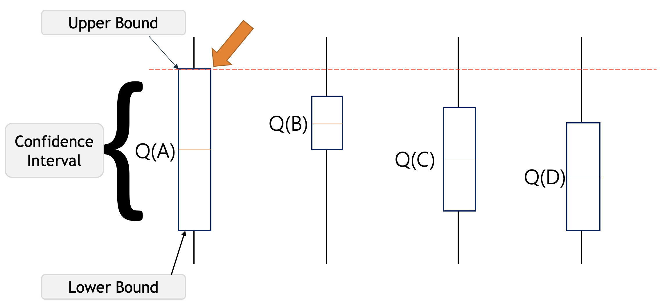
The idea is we the action for which the action value plus the highest possible uncertainty give the highest sum. We are being optimistic in assuming this choice will give the highest reward. In reality any value in the confidence interval could be the true value. Each time we select an action we reduce the uncertainty in the exploration term and we also temper our optimism of the upper confidence bound by the number of times we have selected the action. This means that we will prefer to visit the actions that have not been visited as often.

The main advantage of UCB is that it is more efficient than epsilon greedy in the long run. If we measure the cost of learning in terms of the regret - the difference between the expected reward of the optimal action and the expected reward of the action we choose. UCB has a lower regret than epsilon greedy. The downside is that it is more complex and requires more computation.

\begin{algorithm} \caption{UCB(K, α, β)}\begin{algorithmic} \For{$t = 1, 2, . . .$} \For { $k = 1, . . . , K$ } \State \Comment{ $\textcolor{blue}{compute\ UCBs}$} \State $U_k = \hat\theta_k + c \sqrt{\frac{\ln t}{N_k}}$ \EndFor \State \Comment{ $\textcolor{blue}{select\ and\ apply\ action}$} \State $x_t \leftarrow \arg\max_k h(x,U_x)$ \State Apply xt and observe $y_t$ and $r_t$ \State \Comment{ $\textcolor{blue}{estimate\ model}$} \For{$k = 1, . . . , K$} \State $\hat\theta_k \leftarrow a_k / (α_k + β_k)$ \EndFor \State \Comment{ select and apply action:} \State $x_t \leftarrow \arg\max_k \hat{\theta}_k$ \State Apply $x_t$ and observe $r_t$ \State \Comment{ update distribution:} \State $(α_{x_t}, β_{x_t}) \leftarrow (α_{x_t} + r_t, β_{x_t} + 1 − r_t)$ \EndFor \end{algorithmic} \end{algorithm}

Note we can model UCB using an urn model.

Thompson Sampling

Thompson sampling is basically like UCB but taking the Bayesian approach to the bandit problem. We start with a prior distribution over the action values and then update this distribution as we take actions. The action we choose is then sampled from the posterior distribution. This has the advantage that it is more robust to non-stationary problems than UCB. The downside is that it is more computationally expensive.

Thompson Sampling Algorithm

The algorithm is as follows:

\begin{algorithm} \caption{BernTS(K, α, β)}\begin{algorithmic} \For{$t = 1, 2, . . .$} \State \State \Comment{ sample model} \For{$k = 1, . . . , K$} \State Sample $\hat\theta_k \sim beta(α_k, β_k)$ \EndFor \State \Comment{ select and apply action:} \State $x_t \leftarrow \arg\max_k \hat{\theta}_k$ \State Apply $x_t$ and observe $r_t$ \State \Comment{ update distribution:} \State $(α_{x_t}, β_{x_t}) \leftarrow (α_{x_t} + r_t, β_{x_t} + 1 − r_t)$ \EndFor \end{algorithmic} \end{algorithm}

this is a tutorial on Thompson Sampling

Optimism in the face of uncertainty

Optimism in the face of uncertainty: This is a heuristic to ensure initial exploration of all actions by assuming that untried actions have a high expected reward. We then try to exploit them but end up successively downgrading their expected reward when they do not match our initial optimistic assessment.

The downside to this approach is when the space of action is continuous so we can never get to the benefits of exploration.

Awesome RL resources

Let’s list some useful RL resources.

Books

Richard S. Sutton & Andrew G. Barto RL An Introduction
Tor Latimore’s Book and Blog on Bandit Algorithms.
Csaba Szepesvari’s Book

Courses & Tutorials

David Silver’s 2015 UCL Course on RL Video and Slides.
Charles Isbell and Michael Littman A free Udacity course on RL, with some emphasis on game theory proofs, and some novel algorithms like Coco-Q: Learning in Stochastic Games with Side Payments.
Contextual Bandits tutorial video + papers from MS research videos on contextual bandit algorithms.
Interesting papers:
- We discussed how Dynamic Programming can’t handle games like chess. Here are some RL methods that can.
  - Muzero
  - MuZero and
  - EfficentZero code

Coding Bandits with MESA

from tqdm import tqdm
from mesa import Model, Agent
from mesa.time import RandomActivation
import numpy as np



class EpsilonGreedyAgent(Agent):
    """
    This agent implements the epsilon-greedy 
    """

    def __init__(self, unique_id, model, num_arms, epsilon=0.1):
        super().__init__(unique_id,model)
        self.num_arms = num_arms
        self.epsilon = epsilon
        self.q_values = np.zeros(num_arms)  # Initialize Q-value estimates
        self.action_counts = np.zeros(num_arms)  # Track action counts

    def choose_action(self):
        if np.random.rand() < self.epsilon:
            # Exploration: Choose random arm
            return np.random.randint(0, self.num_arms)
        else:
            # Exploitation: Choose arm with highest Q-value
            return np.argmax(self.q_values)

    def step(self, model):
        chosen_arm = self.choose_action()
        reward = model.get_reward(chosen_arm)
        assert reward is not None, "Reward is not provided by the model"
        self.action_counts[chosen_arm] += 1
        self.q_values[chosen_arm] = (self.q_values[chosen_arm] * self.action_counts[chosen_arm] + reward) / (self.action_counts[chosen_arm] + 1)


class TestbedModel(Model):
    """
    This model represents the 10-armed bandit testbed environment.
    """

    def __init__(self, num_arms, mean_reward, std_dev,num_agents=1):
        super().__init__()
        self.num_agents = num_agents
        self.num_arms = num_arms
        self.mean_reward = mean_reward
        self.std_dev = std_dev
        self.env_init()
        #self.arms = [None] * num_arms  # List to store arm rewards
        self.schedule = RandomActivation(self)
        for i in range(self.num_agents):
          self.create_agent(EpsilonGreedyAgent, i, 0.1) 

    def env_init(self,env_info={}):
        self.arms = np.random.randn(self.num_arms)  # Initialize arm rewards

    def create_agent(self, agent_class, agent_id, epsilon):
        """
        Create an RL agent instance with the specified class and parameters.
        """
        agent = agent_class(agent_id, self, self.num_arms, epsilon)
        self.schedule.add(agent)
        return agent

    def step(self):
        for agent in self.schedule.agents:
            chosen_arm = agent.choose_action()
            reward = np.random.normal(self.mean_reward, self.std_dev)
            self.arms[chosen_arm] = reward  # Update arm reward in the model
            agent.step(self)  # Pass the model instance to the agent for reward access

    def get_reward(self, arm_id):
        # Access reward from the stored list
        return self.arms[arm_id]


# Example usage
model = TestbedModel(10, 0, 1)  # Create model with 10 arms
num_runs = 200                  # The number of times we run the experiment
num_steps = 1000                # The number of pulls of each arm the agent takes


# Run simulation for multiple steps
for _ in tqdm(range(num_runs)):
    for _ in range(num_steps):
        model.step()
    model.step()

  0%|          | 0/200 [00:00<?, ?it/s]  4%|▍         | 9/200 [00:00<00:02, 82.44it/s]  9%|▉         | 18/200 [00:00<00:02, 81.74it/s] 14%|█▎        | 27/200 [00:00<00:02, 80.41it/s] 18%|█▊        | 36/200 [00:00<00:02, 81.26it/s] 22%|██▎       | 45/200 [00:00<00:01, 81.54it/s] 27%|██▋       | 54/200 [00:00<00:01, 81.59it/s] 32%|███▏      | 63/200 [00:00<00:01, 80.82it/s] 36%|███▌      | 72/200 [00:00<00:01, 81.00it/s] 40%|████      | 81/200 [00:00<00:01, 81.45it/s] 45%|████▌     | 90/200 [00:01<00:01, 82.27it/s] 50%|████▉     | 99/200 [00:01<00:01, 82.25it/s] 54%|█████▍    | 108/200 [00:01<00:01, 82.12it/s] 58%|█████▊    | 117/200 [00:01<00:01, 82.58it/s] 63%|██████▎   | 126/200 [00:01<00:00, 82.86it/s] 68%|██████▊   | 135/200 [00:01<00:00, 83.51it/s] 72%|███████▏  | 144/200 [00:01<00:00, 84.59it/s] 76%|███████▋  | 153/200 [00:01<00:00, 85.13it/s] 81%|████████  | 162/200 [00:01<00:00, 85.83it/s] 86%|████████▌ | 171/200 [00:02<00:00, 86.16it/s] 90%|█████████ | 180/200 [00:02<00:00, 86.15it/s] 94%|█████████▍| 189/200 [00:02<00:00, 85.50it/s] 99%|█████████▉| 198/200 [00:02<00:00, 84.65it/s]100%|██████████| 200/200 [00:02<00:00, 83.19it/s]

References

Matha White, Adam White. 2020. “Fundmnentrals on Reinforcement Learning.” University of Alberta; url: https://www.coursera.org/learn/fundamentals-of-reinforcement-learning/.

Reuse

CC SA BY-NC-ND

Citation

BibTeX citation:

@online{bochman2022,
  author = {Bochman, Oren},
  title = {The {K-Armed} {Bandit} {Problem}},
  date = {2022-05-02},
  url = {https://orenbochman.github.io/notes/RL/c1-w1.html},
  langid = {en}
}

For attribution, please cite this work as:

Bochman, Oren. 2022. “The K-Armed Bandit Problem.” May 2, 2022. https://orenbochman.github.io/notes/RL/c1-w1.html.