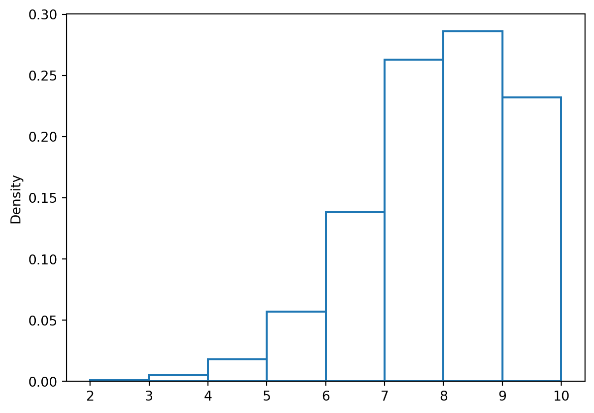
import numpy as np
import matplotlib.pyplot
import seaborn as sns
from collections  import Counter
n_trials = 10
p=3/4
size=1000
x= np.random.binomial(n=n_trials, p=p, size=size)
freqs = Counter(x)
##probs = freqs/size
##print(probs)
##sns.distplot(x, kde=True)
sns.histplot(x, kde=False, stat='density',binwidth=1.0,fill=False)Notes from Udacity A/B Testing course, I took this course around the time it first launched. The course is about planning and analyzing A/B tests - not about implementing A/B testing using a specific framework.
Instructors:
- Carrie Grimes Bostock Googler,
- Caroline Buckey Polaris Googler,
- Diane Tang Googler.
Lesson 1: Overview of A/B Testing
The Instructors gave the following examples of A/B testing from the industry:
- Google tested 41 different shades of blue.
- Amazon initially decided to launch their first personalized product recommendations based on an A/B test showing a huge revenue increase by adding that feature. (See the second paragraph in the introduction.)
- LinkedIn tested whether to use the top slot on a user’s stream for top news articles or an encouragement to add more contacts. (See the first paragraph in “A/B testing with view based JSON” section.)
- Amazon determined that every 100ms increase in page load time decreased sales by 1%. (In “Secondary metrics” section on the last page) Google’s latenc resultsy showed a similar impact for a 100ms delay.
- Kayak tested whether notifying users that their payment was encrypted would make users more or less likely to complete the payment.
- Khan Academy tests changes like letting students know how many other students are working on the exercise with them, or making it easier for students to fast-forward past skills they already have. (See the question “What is the most interesting A/B test you’ve seen so far?”)
- Metrics Difference between click-through rate and click-through probability?
- CTR is used to measure usability e.g. how easy to find the button, \frac{ \text { click}}{\text{ page views}}.
- CTP is used to measure the impact \frac{ \text {unique visitors click}}{\text{ unique visitors view the page}}.
- Statistical significance and practical significance
- Statistical significance is about ensuring observed effects are not due to chance.
- Practical significance depends on the industry e.g. medicine vs. internet.
- Statistical significance
- \alpha: the probability you happen to observe the effect in your sample if H_0 is true.
- Small sample: \alpha low, \beta high.
- Larger sample, \alpha same, \beta lower
- any larger change than your practical significant boundary will have a lower \beta, so it will be easier to detect the significant difference.
- 1-\beta also called sensitivity
- How to calculate sample size?
- Use this calculator, input baseline conversion rate, minimum detectable effect (the smallest effect that will be detected (1-\beta)% of the time), alpha, and beta.
Python Modelling
Binomeal Distribution
Estimate mean and standard deviation
np.set_printoptions(formatter={'float':"{0:0.2f}".format})
np.set_printoptions(precision=2)
mean =  np.round(x.mean(),2)
mean_theoretical =  np.round(n_trials* p,2)
width=6
print(f'mean {mean: <{width}} mean_theoretical  {mean_theoretical}')
variance =  np.round(x.var(),2)
variance_theoretrical =  np.round(n_trials* p * (1-p),2)
print(f'var  {variance: <{width}} var_theoretrical  {variance_theoretrical}')
sd =  np.round(x.std(),2)
sd_theoretical = np.round(np.sqrt(variance_theoretrical),2)
print(f'sd   {sd: <{width}} sd_theoretical    {sd_theoretical}')
##TODO can we do it with PYMC, in a tab
mean 7.47 mean_theoretical 7.5
var 1.89 var_theoretrical 1.88
sd 1.37 sd_theoretical 1.37Estimating p from data
size = 10
n_trials=10
p= np.random.uniform(low=0.0, high=1.0)
x= np.random.binomial(n=n_trials, p=p, size=size)
p=round(p,3)
p_est=np.round(x.mean()/n_trials,3)
p_b_est=np.round((x.mean()+1)/(n_trials+2),3) ## baysian estimator
print(f'{p=} {p_est=} {p_b_est=}')
print(f'\t {np.round(np.abs(p-p_est),3)} {np.round(np.abs(p-p_b_est),3)}')
p=0.971 p_est=0.97 p_b_est=0.892
0.001 0.079Estimating Confidece Intervals
n=n_trials
confidence = 95/100
alpha=1-confidence
z=1-(1/2)*alpha
ci=np.round(z+np.sqrt(p_est*(1-p_est)/n_trials),2)
print(f'{alpha=},{z=}')
print(f'[-{ci},{ci}] wald ci')
z_lb=1-(1/2)*alpha
z_ub=1-(1/2)*(1-alpha)
print(f'{alpha=},{z_lb=},{z_ub=}')
lb_wilson=(p_est+z_lb*z_lb/(2*n)+z_lb*np.sqrt(p_est*(1-p_est)/n + z_lb*z_lb/(4*n)))/(1+z_lb*z_lb/n)
ub_wilson=(p_est+z_ub*z_ub/(2*n)+z_ub*np.sqrt(p_est*(1-p_est)/n + z_ub*z_ub/(4*n)))/(1+z_ub*z_ub/n)
print(f'[-{lb_wilson},{ub_wilson}] wilson ci')
alpha=0.050000000000000044,z=0.975
[-1.03,1.03] wald ci
alpha=0.050000000000000044,z_lb=0.975,z_ub=0.525
[-1.0746188683182163,1.0079729998635674] wilson ciResources
- A/B testing article on Wikipedia.
- These notes were influenced by Joanna
Reuse
CC SA BY-NC-ND
Citation
BibTeX citation:
@online{bochman2023,
  author = {Bochman, Oren},
  title = {Lesson 1 - {Overview} of {A/B} {Testing}},
  date = {2023-01-01},
  url = {https://orenbochman.github.io/notes/AB-testing/l1.html},
  langid = {en}
}
For attribution, please cite this work as:
Bochman, Oren. 2023. “Lesson 1 - Overview of A/B Testing.”
January 1, 2023. https://orenbochman.github.io/notes/AB-testing/l1.html.

