Recurrent Neural Networks for Language Modeling

course banner

This week’s slides

Figure 1

My notes for Week 2 of the Natural Language Processing with Sequence Models Course in the Natural Language Processing Specialization Offered by DeepLearning.AI on Coursera

Learning Objectives

• N-grams
• Gated recurrent units (GRUs)
• Recurrent neural networks (RNNs)

Traditional Language models

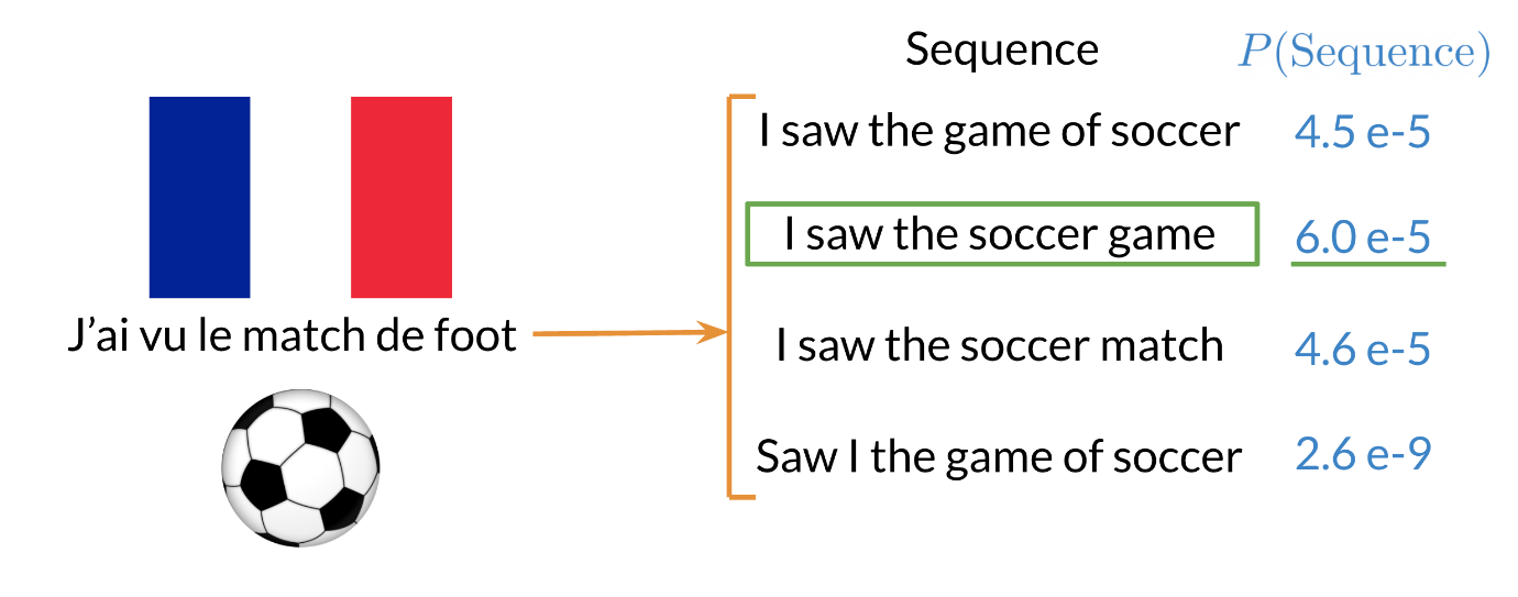
In the example above, the second sentence is the one that is most likely to take place as it has the highest probability of happening. To compute the probabilities, we can do the following:

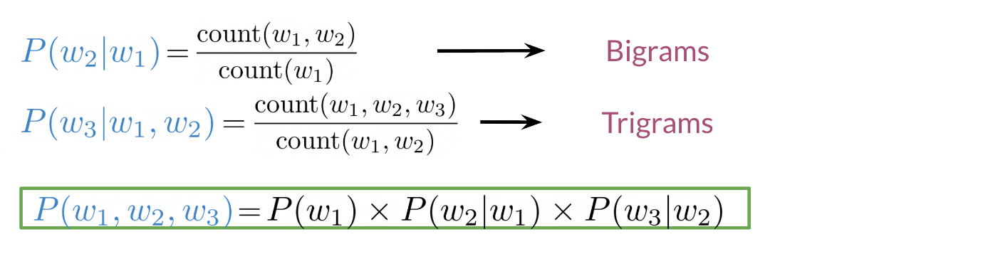
Large N-grams capture dependencies between distant words and need a lot of space and RAM. Hence, we resort to using different types of alternatives.

Recurrent Neural Networks

Previously, we tried using traditional language models, but it turns out they took a lot of space and RAM. For example, in the sentence below:

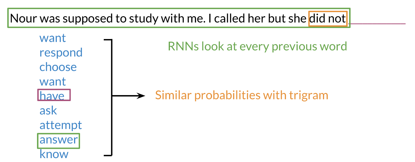
An N-gram (trigram) would only look at “did not” and would try to complete the sentence from there. As a result, the model will not be able to see the beginning of the sentence “I called her but she”. Probably the most likely word is have after “did not”. RNNs help us solve this problem by being able to track dependencies that are much further apart from each other. As the RNN makes its way through a text corpus, it picks up some information as follows:

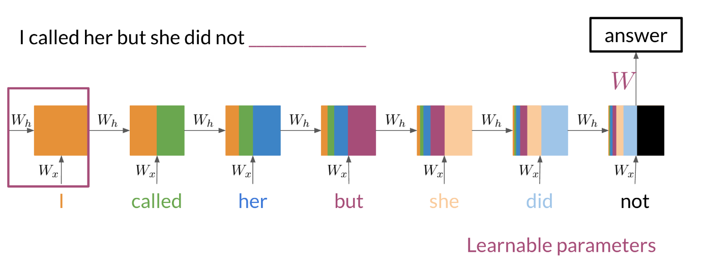
Note that as we feed in more information into the model, the previous word’s retention gets weaker, but it is still there. Look at the orange rectangle above and see how it becomes smaller as we make your way through the text. This shows that your model is capable of capturing dependencies and remembers a previous word although it is at the beginning of a sentence or paragraph. Another advantage of RNNs is that a lot of the computation shares parameters.

Application of RNNs

RNNs could be used in a variety of tasks ranging from machine translation to caption generation. There are many ways to implement an RNN model:

• One to One: given some scores of a championship, we can predict the winner.
• One to Many: given an image, we can predict what the caption is going to be.
• Many to One: given a tweet, we can predict the sentiment of that tweet.
• Many to Many: given an english sentence, we can translate it to its German equivalent.

In the next video, we will see the math in simple RNNs.

Math in Simple RNNs

It is best to explain the math behind a simple RNN with a diagram:

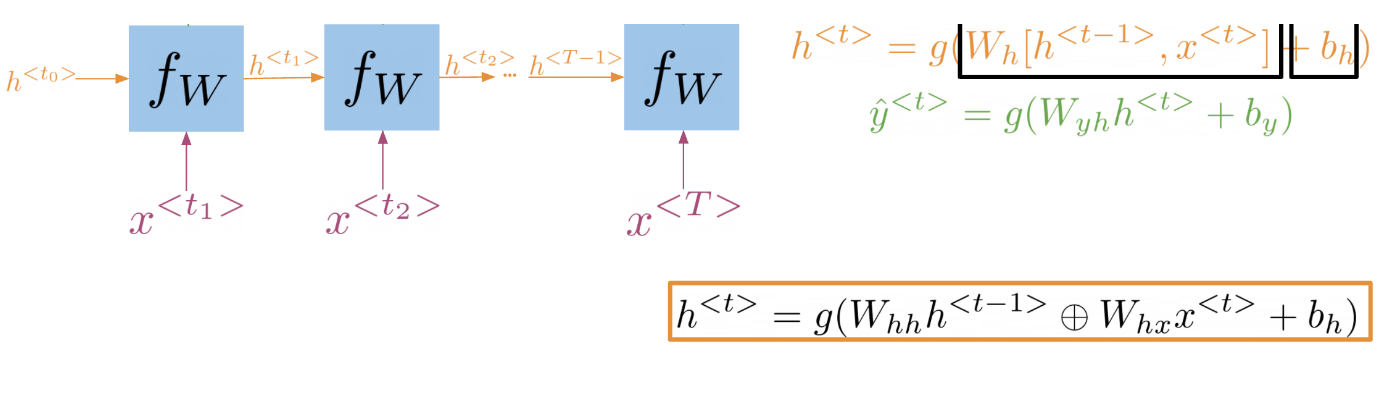
Note that:

h^{<t>} = g(W_{h}[h^{<t-1>}, x^{<t>}] + b_h)

Is the same as multiplying W_{hh} by h and W_{hx} by x. In other words, we can concatenate it as follows:

h^{<t>} = g(W_{hh}[h^{<t-1>} \oplus W_{hx}x^{<t>}] + b_h)

For the prediction at each time step, we can use the following:

\hat{y}^{<t>} = g(W_{yh}h^{<t>} + b_y)

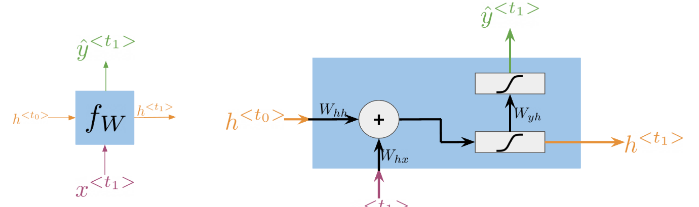
Note that we end up training W_{hh}, W_{hx}, W_{yh}, b_h, and b_y. Here is a visualization of the model.

Lab: Lecture Notebook: Hidden State Activation

Hidden State Activation

Cost Function for RNNs

The cost function used in an RNN is the cross entropy loss. If we were to visualize it

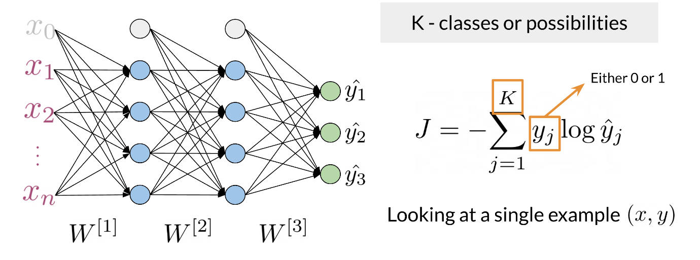
we are basically summing over the all the classes and then multiplying y_j times log(\hat{y}_j). If we were to compute the loss over several time steps, use the following formula:

J = -\frac{1}{T} \sum_{t=1}^{T} \sum_{j=1}^{K} y_j^{<t>} log \hat{y}^{<t>}

where T is the number of time steps and K is the number of classes.

Note that we are simply summing over all the time steps and dividing by T, to get the average cost in each time step. Hence, we are just taking an average through time.

Implementation Note

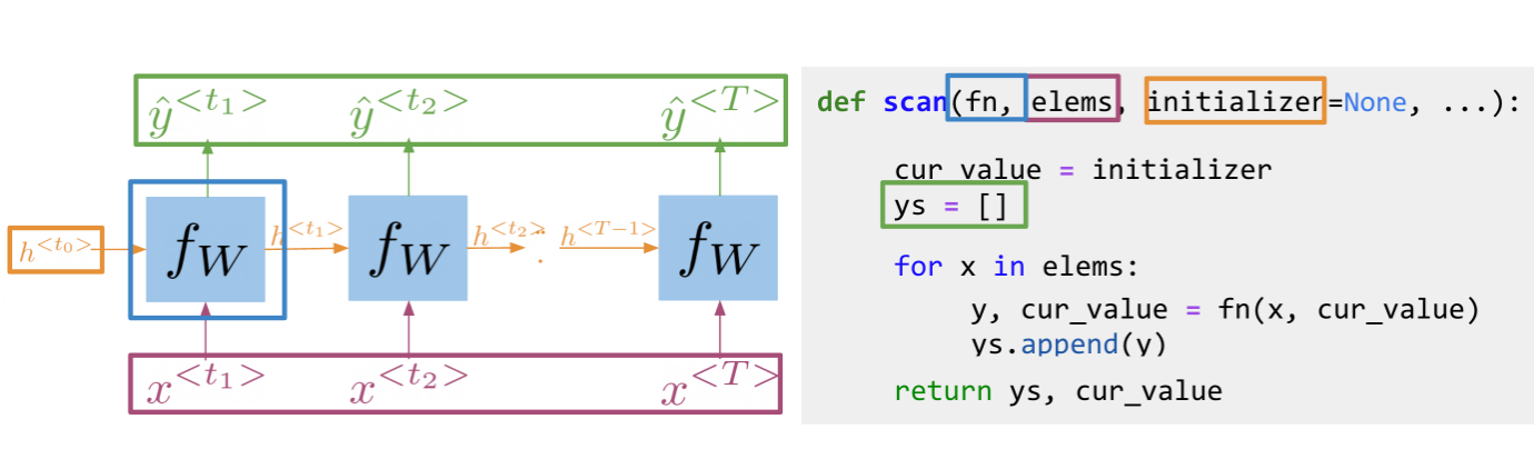
The scan function is built as follows:

Note, that is basically what an RNN is doing. It takes the initializer, and returns a list of outputs (ys), and uses the current value, to get the next y and the next current value. These type of abstractions allow for much faster computation.

Lab: Working with JAX NumPy and Calculating Perplexity

Working with JAX NumPy and Calculating Perplexity

Gated Recurrent Units

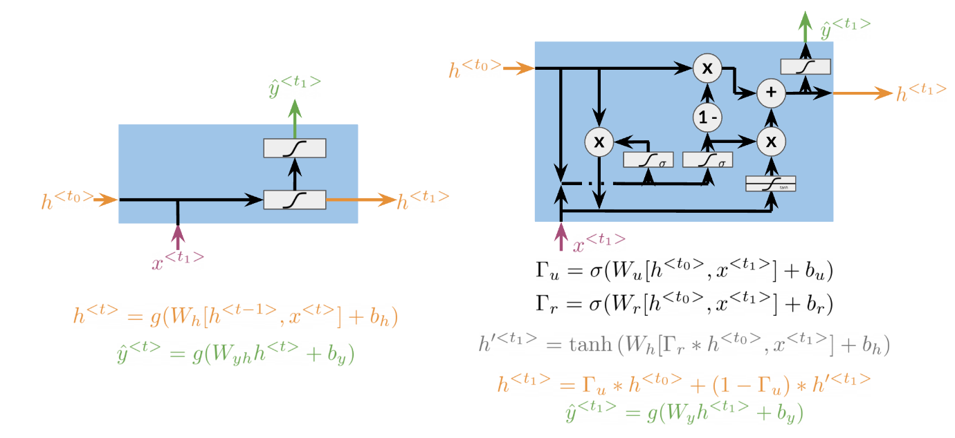
Gated recurrent units are very similar to vanilla RNNs, except that they have a “relevance” and “update” gate that allow the model to update and get relevant information. I personally find it easier to understand by looking at the formulas:

To the left, we have the diagram and equations for a simple RNN. To the right, we explain the GRU. Note that we add 3 layers before computing h and y.

\begin{align*} \Gamma_u &= \sigma(W_u[h^{<t-1>}, x^{<t>}]+b_u) \\ \Gamma_r &= \sigma(W_r[h^{<t-1>}, x^{<t>}]+b_r) \\ h'^{<t>} &= \tanh(W_h[\Gamma_r*h^{<t-1>}, x^{<t>}]+b_h) \\ h^{<t>} &= \Gamma_u*h^{<t-1>} + (1-\Gamma_u)*h'^{<t>} \end{align*}

The first gate Γ_u allows we to decide how much we want to update the weights by. The second gate Γ_r, helps we find a relevance score. We can compute the new h by using the relevance gate. Finally we can compute h, using the update gate. GRUs “decide” how to update the hidden state. GRUs help preserve important information.

Lab: Vanilla RNNs, GRUs and the scan function

Vanilla RNNs, GRUs and the scan function

Lab: Creating a GRU model using Trax

Creating a GRU model using Trax

Deep and Bi-directional RNNs

Bi-directional RNNs are important, because knowing what is next in the sentence could give we more context about the sentence itself.

So we can see, in order to make a prediction \hat{y}, we will use the hidden states from both directions and combine them to make one hidden state, we can then proceed as we would with a simple vanilla RNN. When implementing Deep RNNs, we would compute the following.

Note that at layer l, we are using the input from the bottom a^{[;-1]} and the hidden state h^{<l>} That allows we to get your new h, and then to get your new a, we will train another weight matrix W_{a}, which we will multiply by the corresponding h add the bias and then run it through an activation layer.

Resources:

• (Chadha 2020) Aman Chadha’s Notes
• Ibrahim Jelliti’s Notes

References

Chadha, Aman. 2020. “Distilled Notes for the Natural Language Processing Specialization on Coursera (Offered by Deeplearning.ai).” https://www.aman.ai. www.aman.ai.