we cover Neural networks for deep learning, then build a tweet classifier that places tweets into positive or negative sentiment categories, using a DNN.
NLP
Coursera
notes
Sequence Models
LSTM
Siamese networks
One shot learning
Triplet loss
Author
Oren Bochman
Published
Wednesday, November 18, 2020
Keywords
Cosine similarity, Data generators, Hard negative mining, Modified Triplet Loss, Margin of safety, Cost function for Siamese networks
It is best to describe what a Siamese network is through an example.
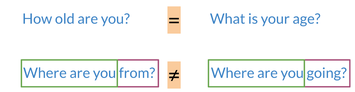
Figure 1: Comparisons questions pairs
Note that in the first example above, the two sentences mean the same thing but have completely different words. While in the second case, the two sentences mean completely different things but they have very similar words.
Classification: learns what makes an input what it is.
Siamese Networks: learns what makes two inputs the same
Here are a few applications of siamese networks:
Figure 2: NLP applications of Siamese Networks include, comparing two signatures, comparing questions or search engine queries,
Video Transcript
In this video you’re going to learn about a special type of neural network known as the Siamese network. It is a neural network made up of two identical neural networks which are merged at the end. This type of architecture has many applications and NLP. And in this video, you’ll see the different examples where you can use it.
Consider the following question. How old are you? And what is your age? You can see that these questions don’t have any words in common. However, they both mean the same thing. On the other hand, if you were to look at the following questions, where are you from? And where are you going? You can see that the first three words are the same. However, the last word completely changes the meaning of each question. This example shows that comparing meaning is not as simple as just comparing words. Coming up, you’re going to see how you can use Siamese networks to compare the meaning of word sequences, and identify question duplicates, which is a very important NLP application at the core of platforms like Stack Overflow or Quora.
Before these platforms allow you to post a new question, they want to be sure that your question hasn’t already been posted by somebody else. Now take this sentence, I’m happy because I’m learning, and consider it in the context of sentiment analysis and binary classification. Now in training a classification algorithm, you discover what features give the statement a positive or negative sentiment.
With Siamese networks you’ll be aiming to identify what’s makes two input similar, and what makes them different. Take a look at these two questions. What is your age? And how old are you? When you build a Siamese model, you’re trying to identify the difference or the similarity between these two questions. You do this by computing a single similarity score, representing the relationship between the two questions. And based on that score when compared against a threshold, you can predict whether these two are the same or different.
Siamese networks have many applications in NLP, you can use them to authenticate handwritten checks by determining whether two signatures are the same or not. You can use them to identify question duplicates on platforms like Quora or Stack Overflow.
And you can use them in search engine queries to predict whether a new query is similar to the one that was already executed. These are just a few examples, but there are many more applications of Siamese networks in NLP.
You can use Siamese networks in many types of NLP applications. In the next video, I’ll walk you through the architecture that is used in this type of model. And I’ll show you how you can use it in a text. I’ll see you in the next video.
Architecture
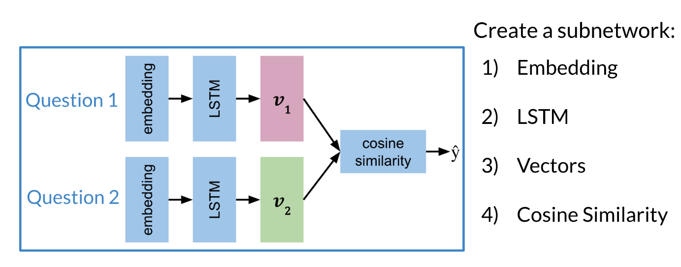
The model architecture of a typical siamese network could look as follows:
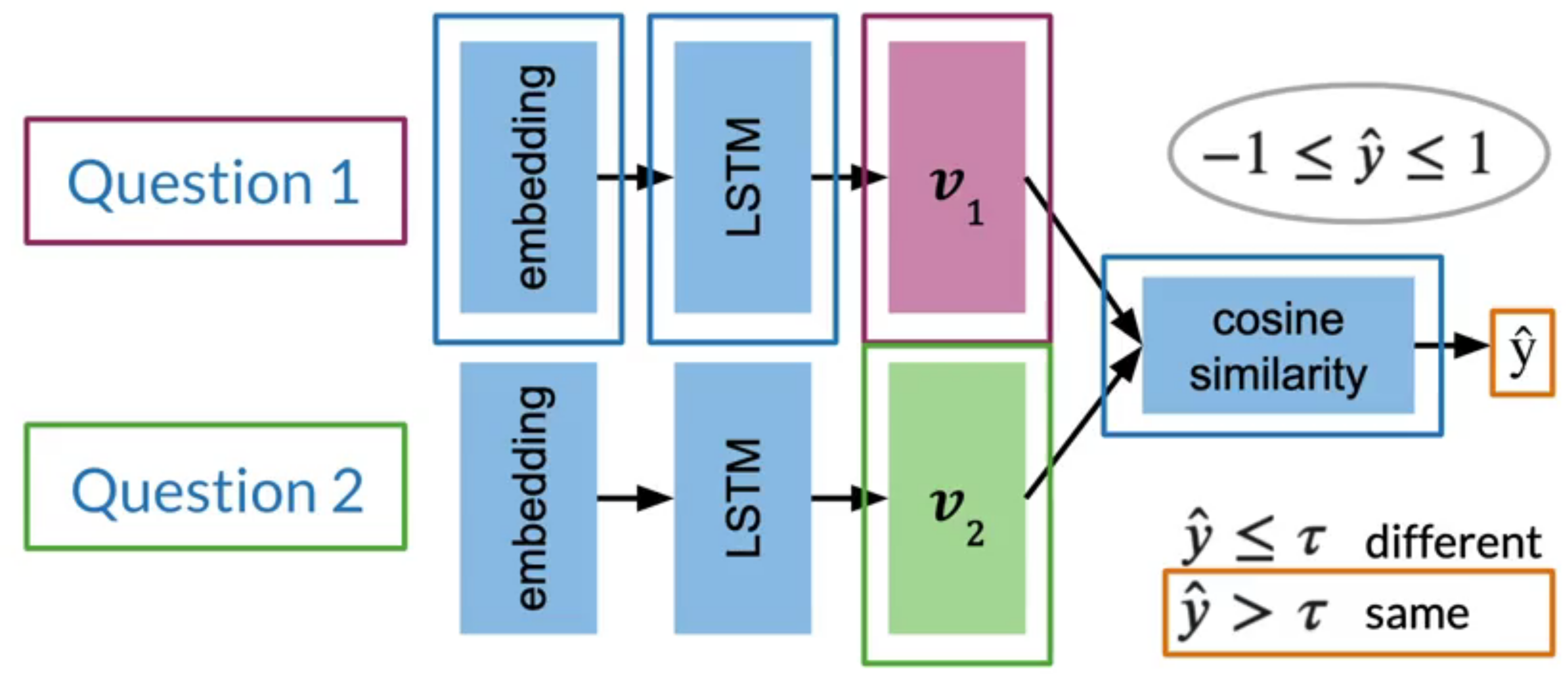
Figure 3: The architecture of a typical siamese network has two sub-networks consisting of embedding LSTMs and a cosine similarity function that evaluates their outputs.
These two sub-networks are sister-networks which come together to produce a similarity score. Not all Siamese networks will be designed to contain LSTMs. One thing to remember is that sub-networks share identical parameters. This means that we only need to train one set of weights and not two.
The output of each sub-network is a vector. We can then run the output through a cosine similarity function to get the similarity score. In the next video, we will talk about the cost function for such a network.
Video Transcript
Siamese networks have a special type of architecture. They have two identical sub-networks which are merged together through a dense layer to produce a final output or its similarity score. I like to think of these two sub-networks as sister-networks which come together to produce a similarity score.
In Figure 3 we can see the model architecture for a Siamese network. Note that the architecture presented here is just an example. Not all Siamese networks will be designed to contain LSTMs.
On the left, you have two inputs which represents Question 1 and Question 2. You will take each question, transform it into an embedding and then you’ll run the embedding through an LSTM layer to model the questions meaning. Each LSTM outputs a vector.
In this architecture, you have two identical sub-networks.
One for Question 1 and the second for Question 2. An important note here is that the sub-networks share identical parameters. That is the learned parameters of each sub-network are exactly the same. So you actually only need to train one sets of weights, not two.
Then given the two outputs vectors, one corresponding to each question, find their cosine similarity.
What is cosine similarity?
Recall that the cosine similarity is a measure of similarity between two vectors. When two vectors point generally in the same direction, the cosine of the angle between them is near one. For vectors that point in opposite directions, the cosine of the angle between them is minus one. If that sounds unfamiliar don’t worry.
Right now you just need to know that the cosine similarity tells you how similar two vectors are. In this case, it tells you how similar the two questions are.
The cosine similarity gives the Siamese networks prediction, denoted here by the variable y-hat, which will be a value between minus one and positive one.
How do we interpret y-hat and tau?
If y-hat is less than or equal to some threshold, tau, then you will say that the input questions are different. If y-hat is greater than tau, then you will say that they are the same.
The threshold tau is a parameter that you will choose based on how often you want to interpret cosine similarity to indicate that two questions are similar or not. A higher threshold means that only very similar sentences will be considered similar.
How would we walking through the architecture
If you think of this process as a series of steps you take to get from your inputs to your outputs, it would go something like this; you start with a model architecture for a Siamese network made up of two identical sub-networks. In this case, your inputs are questions that you feed into each sub-network and each question gets transformed into an embedding and pass through an LSTM layer. Then you take the outputs of each of the sub-networks and compare them using cosine similarity to get your y-hat.
After seeing the model architecture, I’ll start talking about different cost functions you can use for this type of architecture.
Figure 4: Understanding the triplet loss cost function
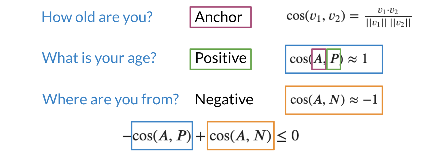
Note that when trying to compute the cost for a siamese network we use the triplet loss. The triplet loss usually consists of an Anchor and a Positive example. Note that the anchor and the positive example have a cosine similarity score that is very close to one. On the other hand, the anchor and the negative example have a cosine similarity score close to -1. Now we are ideally trying to optimize the following equation: −cos(A,P)+cos(A,N)≤0
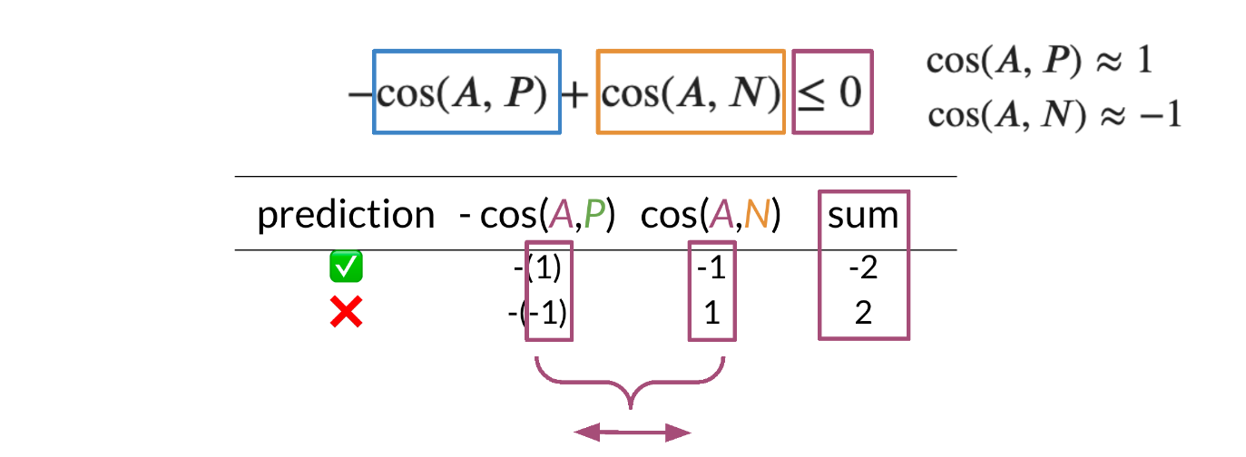
Note that if cos(A,P)=1 is 1 and cos(A,N)=−1, then the equation is definitely less than 0. However, as cos(A,P) deviates from 1 and cos(A,N) deviates from -1, then we can end up getting a cost that is > 0. Here is a visualization that would help we understand what is going on. Feel free to play with different numbers.
Figure 5: A worked example of triplet loss
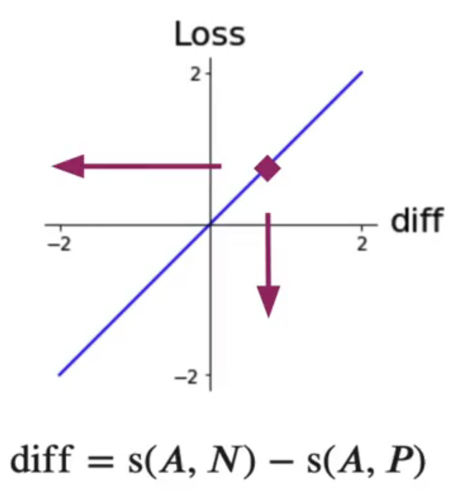
Figure 6: Chart for the loss function
Video Transcript
I’ll now show you a simple loss function you can use in your Siamese network.
Just as a recap, this is the overall structure of the Siamese network, which enables you to predict whether two questions are similar or different, or the outputs of the network, you are able to calculate y-hat, which is the similarity between the two questions.
Now, I’ll show you a loss function for a Siamese network.
What are positive and negative questions?
I’ll starts by looking at this first question, which is, “How old are you?” I’ll call this first question the anchor, which I’m going to use to compare against two other questions relative to the anchor.
Other questions that have the same meaning as the anchor are called positive questions. Whereas questions that do not have the same meaning as the anchor are called negative questions.
Note that the meaning of positive and negative in the context of finding question duplicates is referring to whether a question is similar to the anchor or not, and not whether it has a positive or negative sentiment.
What is a positive question?
The question, “What is your age?” is considered a positive question relative to the anchor, because “How old are you?” and “What is your age?” mean the same thing.
What is a negative question?
This other question, “Where are you from?” is considered a negative question because it does not have the same meaning as the anchor question.
What is cosine similarity?
Here’s a definition of cosine similarity between two vectors. Figure 4 That will be the similarity of function s. To train your model, you’ll be comparing the vectors that are outputs by each sub-network using similarity.
So for this example, you’re going to take the similarity between A and P, where A refers to the anchor question, and P refers to the positive question.
Similarity is bounded between negative one and one. So for vectors that are completely different, the similarity is near negative one, and for vectors that are nearly identical, there similarity is close to positive one.
For a well-trained model, you would like to see a similarity close to one when comparing the anchor and the positive example. Similarly, when comparing the anchor to the negative example, a successful model should yield a similarity close to negative one.
How do you compute the loss?
To begin building a loss function, you start with the similarity of A and N and subtract the similarity of A and P to calculate the difference.
What you have here Figure 6 is a loss function that allows you to determine whether your model is roughly doing what you hope it will do.
Namely, finding that the anchor and the positive example are similar, and that the anchor and the negative example are different.
As the difference gets bigger or smaller along the x-axis, the loss gets bigger or smaller along the y-axis.
When minimizing the loss in training, you are in effect minimizing this difference. You’ve started seeing a difference approach which will allow you to build a different cost function.
Triplets
We will now build on top of our previous cost function. To get the full cost function we will add a margin.
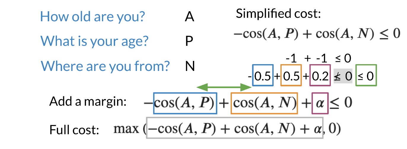
Figure 7: Adding a margin to the triplet loss
Note that we added an α in the equation above. This allows we to have a margin of “safety”.
When computing the full cost, we take the max of that the outcome of −cos(A,P)+cos(A,N)+α and 0. Note, we do not want to take a negative number as a cost.
You will now explore triplets. You’ll see how you can build pairs of inputs. Rather than just classifying what’s an input is, you’re going to build something that will allow you to identify the difference between two inputs. Let’s see how this works.
Here are three questions where the first one, how old are you, is the anchor. The second one is a positive example, what is your age? The third one, where are you from? is a negative example.
Having the three components here is what gives rise to the name triplets, which is to say, an anchor being used in conjunction with a positive and negative pairing. Accordingly, triplet loss is the name for a loss function that uses three components. The intuition behind this simple function is to minimize the difference between the similarity of A and N, and the similarity of A and P. You already know that, as the difference gets bigger or smaller along the x axis, the loss gets bigger or smaller along the y axis.
Do we want the loss to be less than zero?
But notice, when the difference is less than zero, do you also want the loss to be less than zero? Let’s think about this for a moment.
If you gave the model a positive loss value, the model uses this to update its weight to improve.
If you gave the model a negative loss value, this is like telling the model, “Good job. Please update your weight to the worst next time.”
So you don’t actually want to give the model a loss value that’s less than zero. In other words, when the model is doing a good job, you don’t want it to undo a its update. To make sure that the model doesn’t update itself to do worse, you can modify the loss so that whenever the diff is less than zero, the loss should just be zero. When the loss is zero, we’re effectively not asking the model to update it’s weights, because it is performing as expected for that training example. The loss-function now cannot take on negative values. If the difference is less than or equal to 0, the loss is 0. If the difference is greater than 0, then the loss is equal to the difference.
Notice the non-linearity happens at the origin of this line chart.
But you might also wonder what’s happens when the model is correct but only by a tiny bits? The model is still correct if the difference is a tiny number, that is less than zero.
What if you want the model to still learn from this example, and ask it to predict a wider difference for this training example?
You can think of shifting this loss function a little to the left, by a margin that we’ll refer to as Alpha. Let’s say we chose Alpha to be 0.2, if the difference between similarities is very small, like negative 0.1, then if you add it to the Alpha of 0.2, the result is still greater than 0. The sum of the diff plus Alpha can be considered a positive loss that tells the model to learn from this example.
You can see this visually in the line chart. The loss function is shifted to the left by the amount Alpha. The diff is along the horizontal axis. When the difference is less than zero but small in magnitude, the loss is greater than zero. So if the difference is smaller in magnitude than Alpha, then there is still a loss. This loss tells the model that it can still improve and learn from this training example. Triplet loss, as the difference with a margin Alpha, is what you will implement in the assignments which you will code like this, which is the triplet loss function for A, P and N. A small detail worth noting.
In these explanations, I’ve been using similarity because that’s what will be used in the programming assignments, so similarity of v_1, v_2.
But if you were to read the literature, you might find d of v_1, v_2 used also, where this d could be any function that calculates the distance between two vectors. A distance metric is the mirror image of a similarity metric, and a similarity metric can be derived from a distance metric.
One example of a distance metric is Euclidean distance.
How do we pick good triplets?
Selecting triplets A, P, and N for training involves two steps; first, select a pair of questions that are known to be duplicates to serve as the anchor and positive, and you’ll do this from the training set; second, select a question that is known to be difference in meaning from the anchor, to form the anchor and the negative pair.
Why not use random triplets?
If you were to select triplets at random, you’d be likely to select non-duplicative pairs A and N, where the loss is 0.
The loss is zero whenever the model correctly predicts that A and P are more similar relative to A and N.
When the loss is 0, the network has nothing more to learn from the triplets example. So we can train more efficiently if we choose triplets that show the model when it’s incorrect, so that’s just going to adjust it’s weight and improve.
What are hard triplets?
Instead of selecting random triplets, you’ll specifically select so-called hard triplets. That is, triplets that are more difficult to train on. Hard triplets are those where the similarity between anchor and negative is very close to, but still smaller than the similarity between anchor and positive. When the model encounters a hard triplet, the learning algorithm needs to adjust its weight, so that’s it’s going to yield similarities that line up with the real-world labels. So by selecting hard triplets, focusing the training on doing better, on the difficult cases, that it’s predicting incorrectly.
I spoke about easy and hard triplets. I also spoke about a margin. In the next video, you’ll see how all these concepts come together to help us create a cost function.
Computing the Cost I
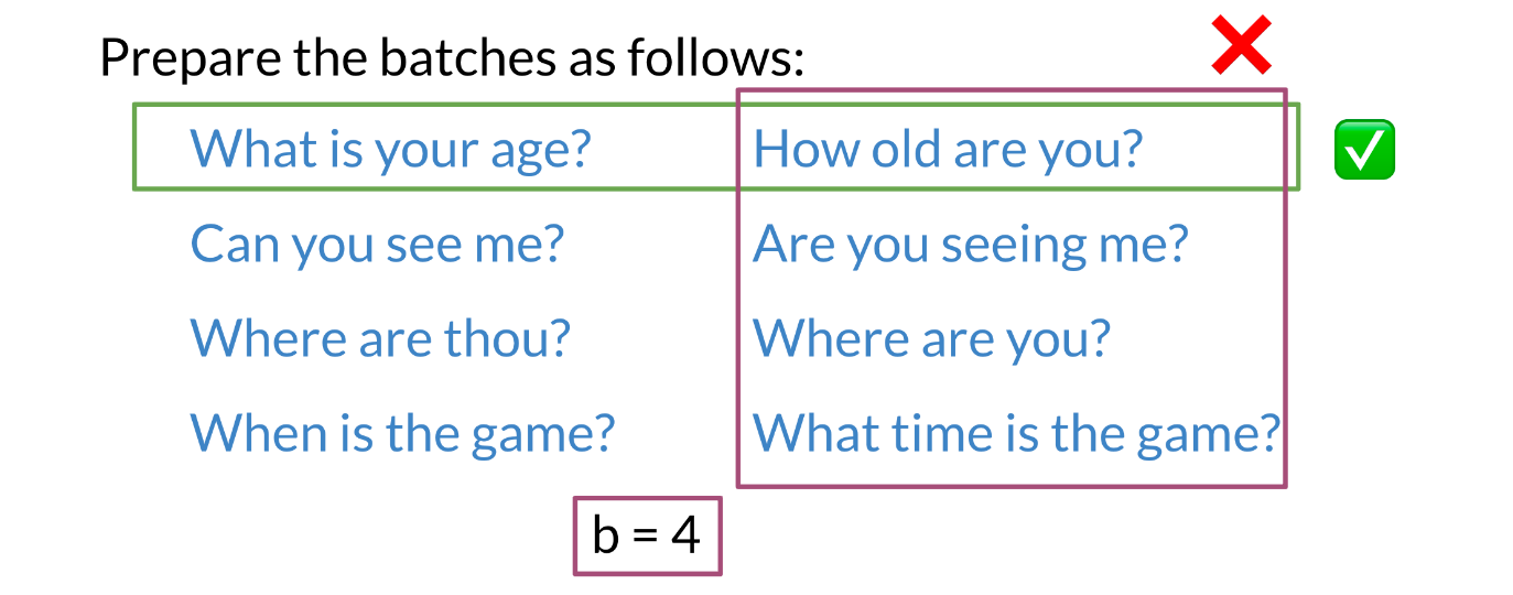
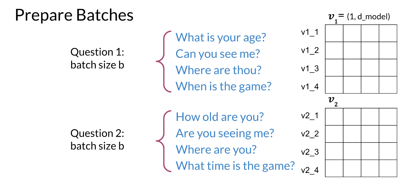
To compute the cost, we will prepare the batches as follows:
Figure 8: An example batch of question pairs
Note that each example, has a similar example to its right, but no other example means the same thing. We will now introduce hard negative mining.
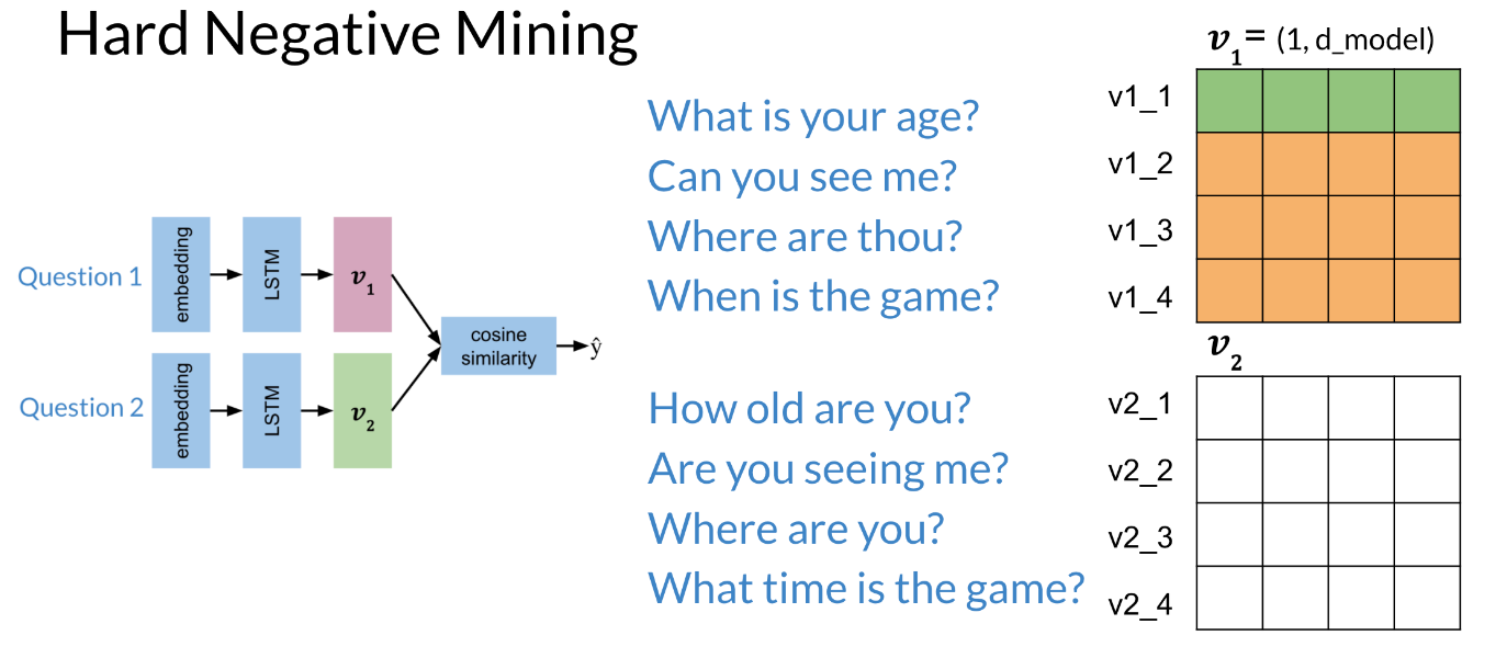
Figure 9: Hard negative mining
Each horizontal vector corresponds to the encoding of the corresponding question. Now when we multiply the two matrices and compute the cosine, we get the following:
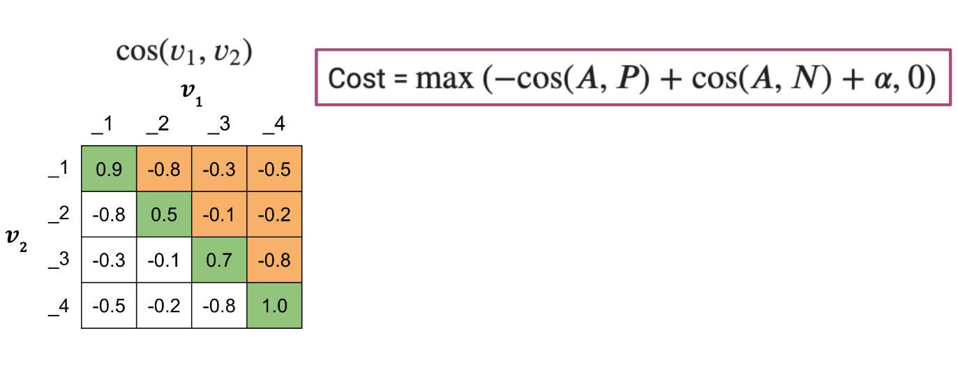
Figure 10: Understanding Cost matrix for a batch of question pairs
The diagonal line corresponds to scores of similar sentences, (normally they should be positive). The off-diagonals correspond to cosine scores between the anchor and the negative examples.
Video Transcript
Welcome back. As promised, you’ll see how everything fits together now. You will start by building a cost function, and then you will use gradient descent to optimize this cost function. Let’s take a look at how this works. To compute the cost, begin by preparing the data in batches. Here you have the questions, what is your age and how old are you? You can see these are duplicates, because they mean the same thing. Can you see me and are you seeing me? Are also duplicates. Where are thou and where are you? Are duplicates too. As are, when is the game and what time is the game? So with four pairs, you have batch size of four. Here we will use the letter b to stand for batch size. Something that’s very important to note is that each question has its corresponding duplicate to the left or right of it. That is, in each row all of the sentences in the columns are duplicates. But you will notice that each question has no duplicates above or below it. That is, for any column, none of the rows in those column contain a sentence that is a duplicate of another sentence in those column. So this is how you prepare the batches. Now, let me show you how you will want to organize the data in this way. Given the first batch, you’re going to run it through this model to get a vector v_1 with dimensions one row by five columns. The number of columns shown in this matrix is equal to the dimension of your embedding layer, which in this case is five. I’ll refer to this dimension of the embedding layer as d model for each question in the batch. I haven’t talked about the dimension of the embedding layer yet, but don’t worry, it will become more clear once you’re working with the code. The important takeaway is that the dimension of the embedding, the model, is a parameter that determines the dimensions of the weights through each layer in the model, and thus determines the size of the outputs vector. The model is running a batch size that is greater than one. So the v_1 outputs is actually a matrix of stacked vectors like this. In this visual example, there are four rows in this matrix to indicate that there are four observations in this batch. The batch size is four. Our subscript to observations in the batch as v_1_1, v_1_2, and so on corresponding to the vector outputs for each question in the batch. You’ll do the same thing for the batch of v_2 vectors. Each question in the batch 1 is a duplicate of its corresponding question in batch 2. But none of the questions in batch 1 are duplicates of each other. The same applies to batch 2. Here, for example, v_1_1 is a duplicate of v_2_1, as are the rest of the respective row pairs. But v_1_1 is not a duplicates of any other rows in v_1. The last step is to combine the two branches of the Siamese network by calculating the similarity between all vector pair combinations of v_1 with v_2. For this example with a batch size of four, you might get a matrix of similarities that looks like this. The diagonal is a key feature here. These values are the similarities for all your positive examples, the question duplicates. Notice that all the values are generally greater than the numbers in the off diagonals. So the model is performing as you would expect for duplicates questions, because you would expect that the question duplicates to have higher similarity compared to the non-duplicates. In the upper right and lower left, you have the similarities for all the negative examples. These are the results for the non-duplicates pairs. Notice that most of these numbers are lower than the similarities that’s are along the diagonal. Also notice that you can have negative example question pairs that still have a similarity greater than zero. The range of similarity ranges from negative 1 to positive 1, but there isn’t any special requirements that a similarity greater than zero indicates duplicates or that’s a similarity less than zero indicates non-duplicates. What’s matters for a properly functioning model is that it generally finds that duplicates have a higher similarity relative to non-duplicates. Creating non-duplicates pairs like this removes the need for additional non-duplicate examples and the input data, which turns out to be a big deal. Instead of needing to sets up specific batches with negative examples, your model can learn from them in the existing question duplicates batches. Now, you can just stop here and use these similarities with the triplet loss function you already know shown here. Then the overall costs for your Siamese network will be the sum of these individual losses over the training sets. Here you can see that superscripts i refers to a specific training example and there are m observations, but there are more techniques available that’s can vastly improve upon model performance. I’ll show you those next.
Computing the Cost II
Now that we have the matrix with cosine similarity scores, which is the product of two matrices, we go ahead and compute the cost.
Figure 11
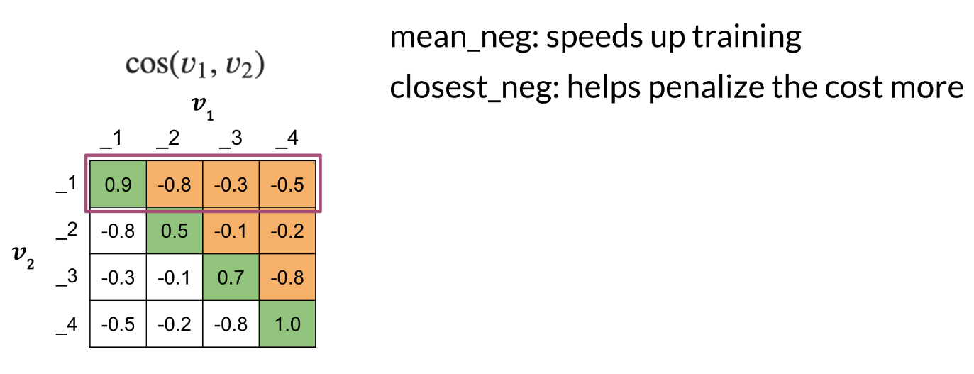
We now introduce two concepts, the mean_neg, which is the mean negative of all the other off diagonals in the row, and the closest_neg, which corresponds to the highest number in the off diagonals.
Cost = \max(−\cos(A,P)+\cos(A,N)+α,0)
So we will have two costs now:
Cost_1 = \max(−\cos(A,P)+ mean_n eg + α,0)
Cost_2 = \max(−\cos(A,P)+ closest_n eg + α,0)
The full cost is defined as: Cost1 + Cost2.
Video Transcript
Previously, you set up the training data into two specific batches, each batch containing no duplicate questions within it. You ran those batches through one sub network each. And that’s produced a vector of supports per question. Which has dimension 1 by d_model, where d_model is the embedding dimension. And is equal to the number of columns in the matrix, which is five, at least in this example. The v_1 vectors for a single batch are stuck together. And in this case, the batch size is the number of rows shown in this matrix, which is four. You can see a similar batch of v_2 vectors as well. The last step was to combine the two branches of the Siamese network. By calculating the similarity between all vector pair combinations of the v_1 vectors and v_2 vectors. For this example with a batch size of four, that last step would produce a matrix of similarities that looks something like this.
What are the attributes of this matrix?
This matrix has some important attributes. The similarities along the green diagonal contain similarities for the duplicate questions. For a well trained model, these values should be greater than similarities for the off-diagonals. Reflecting the fact that the network produces similar vector outputs for duplicate questions. The orange values in the upper right and lower left are similarities for the non duplicate questions.
Now this is where things get really interesting. You can use this off diagonal information to make some modifications to the loss function and really improve your models performance. To do so, I’m going to make use of two concepts.
What is the mean negative?
The first concept is the mean negative, which is just the mean or average of all the off-diagonal values in each row. Notice that off-diagonal elements can still be positive numbers. So when I say mean negative, I’m referring to the mean of the similarity for negative examples, not the mean of negative numbers in a row.
For example, the mean negative of the first row is just the mean of all the off-diagonal values in that row.
In this case, -0.8, 0.3 and -0.5, excluding the value 0.9, which is on the diagonal. You can use the mean negative to help speed up training by modifying the loss function, which I’ll show you soon.
What is the closest negative?
The next concept is what’s called the closest negative. As mentioned earlier, because of the way you define the triplet loss function, you’ll need to choose so called hard triplets to train on. What this means is that for training, you want to choose triplets where the cosine similarity of the negative example is close to the similarity of the positive example.
This forces your model to learn what differentiates these examples and ultimately drive those similarity values further apart through training. To do this, you’ll search each row in your output matrix for the closest negative. Which is to say the off diagonal value which is closest to, but still less than the value on the on diagonal for that row. So in this first row, the value on the diagonal is 0.9. So the closest off-diagonal elements in this case is 0.3. What this means is that this negative example with a similarity of 0.3 has the most to offer your model in terms of learning opportunity.
How do we use these new concepts ?
To make use of these new concepts, recall that the triplet loss was defined as the max of the similarity of A and N minus the similarity of A and B plus the margin alpha and 0. Also recall that we refer to the difference between the two similarities with the variable named diff.
Here, we’re just writing out the definition of diff. So in order to minimize the loss you want this diff plus the margin alpha to be less than or equal to 0. I’ll introduce loss 1 to be the max of the mean negative minus the similarity of A and P plus alpha and 0. The change between the formulas for triplet loss and loss 1 is the replacement of similarity of A and N. With the mean negative, this helps the model converge faster during training by reducing noise. It reduces noise by training on just the average of several observations, rather than training the model on each of these off-diagonal examples.
So why does taking the average of several observations usually reduce noise? Well, we define noise to be a small value that comes from a distribution that is centered around 0. So in other words, the average of several noise values is usually 0. So if we took the average of several examples, this has the effect of cancelling out the individual noise from those observations. Then loss 2 will be the max of the closest negative minus the similarity of A and B plus alpha and 0.
The difference between the formulas this time is the replacement of the cosine of A and N. With the closest negative, this helps create a slightly larger penalty by diminishing the effects of the otherwise more negative similarity of A and N that it replaces.
You can think of the closest negative as finding the negative example that results in the smallest difference between the two cosine similarities. If you had that small difference to alpha, then you’re able to generate the largest loss among all of the other examples in that row.
By focusing the training on the examples that produce higher loss values, you make the model update its weights more.
To learn from these more difficult examples, then you can define the full loss as loss 1 + loss 2. And you will use this new full loss as an improved triplet loss in the assignments. The overall costs for your Siamese network will be the sum of these individual losses over the training sets.
In the next video, you will use this cost function in one shot learning. One shot learning is a very effective technique that can save you a lot of time when comparing the authenticity of checks or of any other type of inputs
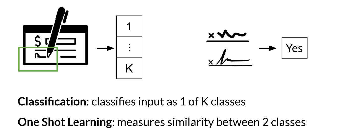
Imagine we are working in a bank and we need to verify the signature of a check. We can either build a classifier with K possible signatures as an output or we can build a classifier that tells we whether two signatures are the same.
Figure 12: Classification vs one shot learning
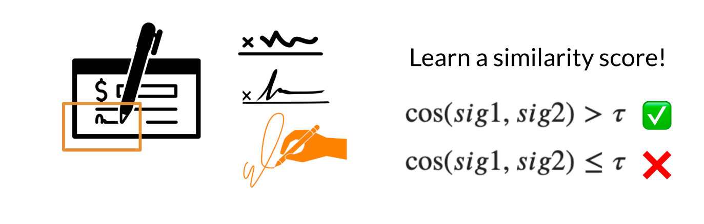
Hence, we resort to one shot learning. Instead of retraining your model for every signature, we can just learn a similarity score as follows:
Figure 13
Video Transcript
Let’s say that you’re trying to identify whether the author for a certain poem is Lucas or not. You can either take all of Lucas’ poems and put them into datasets, and instead of predicting K classes, you will now predict K plus 1 classes. All the previous poems of other authors plus Lucas’, so that’s why it’s k plus 1. Or you can compare one of Lucas’ poems to another poem, and that is where one-shot learning comes in. In this video, I’ll show you how you can do that. To understand the difference between classification and one-shot learning, first consider identifying or classifying signatures based on one through K possible classes. You might use some classification model trained on the K classes, probably with a softmax function at the end to find the maximum probability. Then at recognition time, classify the input signature to one of those corresponding classes. That’s great if you have a signature list that’s rarely changes. But what if you get a new signature to classify? It would be expensive to retrain the model every time this happens, and besides, unless you have a great many examples of that new signature, model training won’t work very well. In one-shot learning, you need to be able to recognize a signature repeatedly from just one example. You can do this with a learned similarity function. Then you can test a similarity score against some threshold to see if two signatures are the same. So the problem changes to determining which class to instead measuring similarity between two classes. This is very useful, especially in banks, for example. Every time there’s a new signature, you can’t retrain your entire system to classify the signatures into K possible outputs. So instead, you just learn a similarity function that can be used to calculate a similarity score. That can in turn be used to identify whether two signatures are the same. You already did this using cosine similarity as the similarity function. If the result was greater than some threshold Tau, you determine the inputs to be the same. In the case of comparing signatures, if the similarity is less than or equal to Tau, then the signatures are different. In this video, I spoke about one-shot learning and I told you why it is a very effective technique. One-shot learning makes use of Siamese networks. In the next video, I’ll show you how you can train and test your Siamese network.
Training and Testing
After preparing the batches of vectors, we can proceed to multiplying the two matrices.
Here is a quick recap of the first step:
Figure 14: Preparing batches of questions
The next step is to implement the siamese model as follows:
Figure 15: Reviewing the architecture of the siamese networks
Finally when testing:
Convert two inputs into an array of numbers
Feed it into your model
Compare 𝒗_1,𝒗_2 using cosine similarity
Test against a threshold \tau
Video Transcript
In this video, you’re goingto see what the dataset would look like for a Siamese network. I’ll show you how you can train your model and then you can use that model to test your Siamese network. Let’s take a look at how you can do this. You’ll be using the Quora question duplicates datasets for this week’s programming assignment. It looks like this. It consists of a collection of question pairs within its duplicates Boolean for each question. For example, for Question 1 and Question 2, “What is your age?” and “How old are you?” Its duplicate equals “true” because these two questions are duplicates. “Where are you from?” and “Where are you going?” are not duplicates, so it’s false and so on. This dataset gives your model plenty of examples to learn from. First, you will process the dataset so that it looks like this. You will pre-process the data into batches of size b. The corresponding questions from each batch are duplicates. For example, the first question in Batch 1, “What is your age?” is a duplicate of the first question in Batch 2, “How old are you?” The second question in Batch 1 is a duplicate of the second question in Batch 2 and so on.
Note however, that there are no duplicates within an individual batch. If I call this q1_a, this q2_a, then q1_a and q2_a are duplicates. If this was q1_b and this was q2_b, then q1_b and q2_b are duplicates. However, q1_a and q1_b are not duplicates. Similarly, q2_a and q2_b are not duplicates. I’ll show you how to prepare the batches in such a way that no question within the same batch is duplicated. Finally, you’ll use these inputs to get outputs vectors for each batch. Then, you can calculate the cosine similarity between each pair of output vectors. This is the Siamese model that you’ll be implementing in the assignment. You’ll create a subnetwork, which is then duplicated and drawn in parallel. In each subnetwork, you got the embedding, run it through the LSTM, take your vector output, and then use them to find the cosine similarity.
An important note here, is that the learned parameters of the subnetworks are exactly the same between the two subnetworks. So you are actually only training one sets of weights, not two. When testing the model, you will perform one-shot learning. The goal is to find a similarity score between two inputs questions. First, convert each input into an array of numbers. Feed these into your model. Compare the subnetwork outputs v_1 and v_2 using cosine similarity for a similarity score. Then, test the score against some threshold Tau, and if the cosine similarity is greater than Tau, then the questions are classified as duplicates.
Note that both $tau$ and the margin \alpha from the last function are tunable hyperparameters.
Congratulations, you now know how to train your Siamese network and you know how to test it. In this week’s programming exercise, you’ll be using a Siamese network to identify whether a question is a duplicate or not. Specifically, you’ll be using the Quora question duplicate data sets, and using that, you’ll be able to get a very good accuracy.
Could we improve the model by Can we give each LSTM it own loss function?
What are some typical use cases for using Siamese networks?
Face recognition. The faces are very different from each other but we don’t want to retrain the model for every new face - we typically want to check if a face is the same as one of the faces on file.
Signature verification is a good example of a use case for Siamese networks. We want to check if a signatures we get is sufficiently similar to the few samples we have on file.
One shot learning is another area where Siamese networks could be useful.
In which NLP tasks are Siamese networks utilized?
Search engine queries are often challenging since they are very brief compared to the documents they are searching for, and so they tend to miss the best variation for some query. Also the distribution has many similar queries and a long tail of unique queries.
Question-Answering sites like Stack overflow or Quora is another place where Siamese networks could be useful. The crowd sourcing works better if the questions are not repeated so that all the answers are in one place.
Paraphrase detection is another area where Siamese networks could be useful. The paraphrase could be a completely different sentence but the meaning remains the same.
Spam detection is another area where Siamese networks could be useful. The spammer could change the words in the spam message but the meaning remains the same.
How can we improve the model by using a different similarity function?
Are there any benefits to use Location sensitive hashing with the cosine similarity function ?
Chadha, Aman. 2020. “Distilled Notes for the Natural Language Processing Specialization on Coursera (Offered by Deeplearning.ai).”https://www.aman.ai. www.aman.ai.
Citation
BibTeX citation:
@online{bochman2020,
  author = {Bochman, Oren},
  title = {Siamese {Networks}},
  date = {2020-11-18},
  url = {https://orenbochman.github.io/notes-nlp/notes/c3w4/},
  langid = {en}
}