Word Embeddings: Training the CBOW model

course banner

In previous lecture notebooks we saw

1. how to prepare data before feeding it to a continuous bag-of-words model,
2. the model itself, its architecture and activation functions.

This notebook will walk we through:

• Forward propagation.
• Cross-entropy loss.
• Backpropagation.
• Gradient descent.

Which are concepts necessary to understand how the training of the model works.

Let’s dive into it!

import numpy as np
from utils2 import get_dict

Forward propagation

Let’s dive into the neural network itself, which is shown below with all the dimensions and formulas you’ll need.

Figure 1

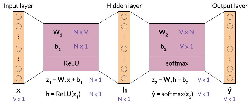
Set N equal to 3. Remember that N is a hyperparameter of the CBOW model that represents the size of the word embedding vectors, as well as the size of the hidden layer.

Also set V equal to 5, which is the size of the vocabulary we have used so far.

# Define the size of the word embedding vectors and save it in the variable 'N'
N = 3

# Define V. Remember this was the size of the vocabulary in the previous lecture notebooks
V = 5

Initialization of the weights and biases

Before we start training the neural network, we need to initialize the weight matrices and bias vectors with random values.

In the assignment we will implement a function to do this yourself using numpy.random.rand. In this notebook, we’ve pre-populated these matrices and vectors for you.

# Define first matrix of weights
W1 = np.array([[ 0.41687358,  0.08854191, -0.23495225,  0.28320538,  0.41800106],
               [ 0.32735501,  0.22795148, -0.23951958,  0.4117634 , -0.23924344],
               [ 0.26637602, -0.23846886, -0.37770863, -0.11399446,  0.34008124]])

# Define second matrix of weights
W2 = np.array([[-0.22182064, -0.43008631,  0.13310965],
               [ 0.08476603,  0.08123194,  0.1772054 ],
               [ 0.1871551 , -0.06107263, -0.1790735 ],
               [ 0.07055222, -0.02015138,  0.36107434],
               [ 0.33480474, -0.39423389, -0.43959196]])

# Define first vector of biases
b1 = np.array([[ 0.09688219],
               [ 0.29239497],
               [-0.27364426]])

# Define second vector of biases
b2 = np.array([[ 0.0352008 ],
               [-0.36393384],
               [-0.12775555],
               [-0.34802326],
               [-0.07017815]])

Check that the dimensions of these matrices match those shown in the figure above.

print(f'V (vocabulary size): {V}')
print(f'N (embedding size / size of the hidden layer): {N}')
print(f'size of W1: {W1.shape} (NxV)')
print(f'size of b1: {b1.shape} (Nx1)')
print(f'size of W2: {W2.shape} (VxN)')
print(f'size of b2: {b2.shape} (Vx1)')

V (vocabulary size): 5
N (embedding size / size of the hidden layer): 3
size of W1: (3, 5) (NxV)
size of b1: (3, 1) (Nx1)
size of W2: (5, 3) (VxN)
size of b2: (5, 1) (Vx1)

Before moving forward, we will need some functions and variables defined in previous notebooks. They can be found next. Be sure we understand everything that is going on in the next cell, if not consider doing a refresh of the first lecture notebook.

# Define the tokenized version of the corpus
words = ['i', 'am', 'happy', 'because', 'i', 'am', 'learning']

# Get 'word2Ind' and 'Ind2word' dictionaries for the tokenized corpus
word2Ind, Ind2word = get_dict(words)

# Define the 'get_windows' function as seen in a previous notebook
def get_windows(words, C):
    i = C
    while i < len(words) - C:
        center_word = words[i]
        context_words = words[(i - C):i] + words[(i+1):(i+C+1)]
        yield context_words, center_word
        i += 1

# Define the 'word_to_one_hot_vector' function as seen in a previous notebook
def word_to_one_hot_vector(word, word2Ind, V):
    one_hot_vector = np.zeros(V)
    one_hot_vector[word2Ind[word]] = 1
    return one_hot_vector

# Define the 'context_words_to_vector' function as seen in a previous notebook
def context_words_to_vector(context_words, word2Ind, V):
    context_words_vectors = [word_to_one_hot_vector(w, word2Ind, V) for w in context_words]
    context_words_vectors = np.mean(context_words_vectors, axis=0)
    return context_words_vectors

# Define the generator function 'get_training_example' as seen in a previous notebook
def get_training_example(words, C, word2Ind, V):
    for context_words, center_word in get_windows(words, C):
        yield context_words_to_vector(context_words, word2Ind, V), word_to_one_hot_vector(center_word, word2Ind, V)

Training example

Run the next cells to get the first training example, made of the vector representing the context words “i am because i”, and the target which is the one-hot vector representing the center word “happy”.

We don’t need to worry about the Python syntax, but there are some explanations below if we want to know what’s happening behind the scenes.

# Save generator object in the 'training_examples' variable with the desired arguments
training_examples = get_training_example(words, 2, word2Ind, V)

get_training_examples, which uses the yield keyword, is known as a generator. When run, it builds an iterator, which is a special type of object that… we can iterate on (using a for loop for instance), to retrieve the successive values that the function generates.

In this case get_training_examples yields training examples, and iterating on training_examples will return the successive training examples.

# Get first values from generator
x_array, y_array = next(training_examples)

next is another special keyword, which gets the next available value from an iterator. Here, you’ll get the very first value, which is the first training example. If we run this cell again, you’ll get the next value, and so on until the iterator runs out of values to return.

In this notebook next is used because we will only be performing one iteration of training. In this week’s assignment with the full training over several iterations you’ll use regular for loops with the iterator that supplies the training examples.

The vector representing the context words, which will be fed into the neural network, is:

# Print context words vector
x_array

array([0.25, 0.25, 0.  , 0.5 , 0.  ])

The one-hot vector representing the center word to be predicted is:

# Print one hot vector of center word
y_array

array([0., 0., 1., 0., 0.])

Now convert these vectors into matrices (or 2D arrays) to be able to perform matrix multiplication on the right types of objects, as explained in a previous notebook.

# Copy vector
x = x_array.copy()

# Reshape it
x.shape = (V, 1)

# Print it
print(f'x:\n{x}\n')

# Copy vector
y = y_array.copy()

# Reshape it
y.shape = (V, 1)

# Print it
print(f'y:\n{y}')

x:
[[0.25]
 [0.25]
 [0.  ]
 [0.5 ]
 [0.  ]]

y:
[[0.]
 [0.]
 [1.]
 [0.]
 [0.]]

Now we will need the activation functions seen before. Again, if this feel unfamiliar consider checking the previous lecture notebook.

# Define the 'relu' function as seen in the previous lecture notebook
def relu(z):
    result = z.copy()
    result[result < 0] = 0
    return result

# Define the 'softmax' function as seen in the previous lecture notebook
def softmax(z):
    e_z = np.exp(z)
    sum_e_z = np.sum(e_z)
    return e_z / sum_e_z

Values of the hidden layer

Now that we have initialized all the variables that we need for forward propagation, we can calculate the values of the hidden layer using the following formulas:

\begin{align} \mathbf{z_1} = \mathbf{W_1}\mathbf{x} + \mathbf{b_1} \tag{1} \\ \mathbf{h} = \mathrm{ReLU}(\mathbf{z_1}) \tag{2} \\ \end{align}

First, we can calculate the value of \mathbf{z_1}.

# Compute z1 (values of first hidden layer before applying the ReLU function)
z1 = np.dot(W1, x) + b1

 np.dot is numpy’s function for matrix multiplication.

As expected we get an N by 1 matrix, or column vector with N elements, where N is equal to the embedding size, which is 3 in this example.

# Print z1
z1

array([[ 0.36483875],
       [ 0.63710329],
       [-0.3236647 ]])

We can now take the ReLU of \mathbf{z_1} to get \mathbf{h}, the vector with the values of the hidden layer.

# Compute h (z1 after applying ReLU function)
h = relu(z1)

# Print h
h

array([[0.36483875],
       [0.63710329],
       [0.        ]])

Applying ReLU means that the negative element of \mathbf{z_1} has been replaced with a zero.

Values of the output layer

Here are the formulas we need to calculate the values of the output layer, represented by the vector \mathbf{\hat y}:

\begin{align} \mathbf{z_2} &= \mathbf{W_2}\mathbf{h} + \mathbf{b_2} \tag{3} \\ \mathbf{\hat y} &= \mathrm{softmax}(\mathbf{z_2}) \tag{4} \\ \end{align}

First, calculate \mathbf{z_2}.

# Compute z2 (values of the output layer before applying the softmax function)
z2 = np.dot(W2, h) + b2

# Print z2
z2

array([[-0.31973737],
       [-0.28125477],
       [-0.09838369],
       [-0.33512159],
       [-0.19919612]])

Expected output:

array([[-0.31973737],
       [-0.28125477],
       [-0.09838369],
       [-0.33512159],
       [-0.19919612]])

This is a V by 1 matrix, where V is the size of the vocabulary, which is 5 in this example.

Now calculate the value of \mathbf{\hat y}.

# Compute y_hat (z2 after applying softmax function)
y_hat = softmax(z2)

# Print y_hat
y_hat

array([[0.18519074],
       [0.19245626],
       [0.23107446],
       [0.18236353],
       [0.20891502]])

Expected output:

array([[0.18519074],
       [0.19245626],
       [0.23107446],
       [0.18236353],
       [0.20891502]])

As you’ve performed the calculations with random matrices and vectors (apart from the input vector), the output of the neural network is essentially random at this point. The learning process will adjust the weights and biases to match the actual targets better.

That being said, what word did the neural network predict?

Solution

The neural network predicted the word “happy”: the largest element of \mathbf{\hat y} is the third one, and the third word of the vocabulary is “happy”.

Here’s how we could implement this in Python:

print(Ind2word[np.argmax(y_hat)])

Well done, you’ve completed the forward propagation phase!

Cross-entropy loss

Now that we have the network’s prediction, we can calculate the cross-entropy loss to determine how accurate the prediction was compared to the actual target.

Remember that we are working on a single training example, not on a batch of examples, which is why we are using loss and not cost, which is the generalized form of loss.

First let’s recall what the prediction was.

# Print prediction
y_hat

array([[0.18519074],
       [0.19245626],
       [0.23107446],
       [0.18236353],
       [0.20891502]])

And the actual target value is:

# Print target value
y

array([[0.],
       [0.],
       [1.],
       [0.],
       [0.]])

The formula for cross-entropy loss is:

J=-\sum\limits_{k=1}^{V}y_k\log{\hat{y}_k} \tag{6}

Try implementing the cross-entropy loss function so we get more familiar working with numpy

Here are a some hints if you’re stuck.

def cross_entropy_loss(y_predicted, y_actual):
    # Fill the loss variable with your code
    loss = np.sum(-np.log(y_predicted)*y_actual)
    return loss

Hint 1

<p>To multiply two numpy matrices (such as <code>y</code> and <code>y_hat</code>) element-wise, we can simply use the <code>*</code> operator.</p>

Hint 2

Once we have a vector equal to the element-wise multiplication of y and y_hat, we can use np.sum to calculate the sum of the elements of this vector.

Solution

loss = np.sum(-np.log(y_hat)*y)

Don’t forget to run the cell containing the cross_entropy_loss function once it is solved.

Now use this function to calculate the loss with the actual values of \mathbf{y} and \mathbf{\hat y}.

# Print value of cross entropy loss for prediction and target value
cross_entropy_loss(y_hat, y)

np.float64(1.4650152923611108)

Expected output:

1.4650152923611106

This value is neither good nor bad, which is expected as the neural network hasn’t learned anything yet.

The actual learning will start during the next phase: backpropagation.

Backpropagation

The formulas that we will implement for backpropagation are the following.

\begin{align} \frac{\partial J}{\partial \mathbf{W_1}} &= \rm{ReLU}\left ( \mathbf{W_2^\top} (\mathbf{\hat{y}} - \mathbf{y})\right )\mathbf{x}^\top \tag{7}\\ \frac{\partial J}{\partial \mathbf{W_2}} &= (\mathbf{\hat{y}} - \mathbf{y})\mathbf{h^\top} \tag{8}\\ \frac{\partial J}{\partial \mathbf{b_1}} &= \rm{ReLU}\left ( \mathbf{W_2^\top} (\mathbf{\hat{y}} - \mathbf{y})\right ) \tag{9}\\ \frac{\partial J}{\partial \mathbf{b_2}} &= \mathbf{\hat{y}} - \mathbf{y} \tag{10} \end{align}

Note: these formulas are slightly simplified compared to the ones in the lecture as you’re working on a single training example, whereas the lecture provided the formulas for a batch of examples. In the assignment you’ll be implementing the latter.

Let’s start with an easy one.

Calculate the partial derivative of the loss function with respect to \mathbf{b_2}, and store the result in grad_b2.

\frac{\partial J}{\partial \mathbf{b_2}} = \mathbf{\hat{y}} - \mathbf{y} \tag{10}

# Compute vector with partial derivatives of loss function with respect to b2
grad_b2 = y_hat - y

# Print this vector
grad_b2

array([[ 0.18519074],
       [ 0.19245626],
       [-0.76892554],
       [ 0.18236353],
       [ 0.20891502]])

Expected output:

array([[ 0.18519074],
       [ 0.19245626],
       [-0.76892554],
       [ 0.18236353],
       [ 0.20891502]])

Next, calculate the partial derivative of the loss function with respect to \mathbf{W_2}, and store the result in grad_W2.

\frac{\partial J}{\partial \mathbf{W_2}} = (\mathbf{\hat{y}} - \mathbf{y})\mathbf{h^\top} \tag{8}

Hint: use .T to get a transposed matrix, e.g. h.T returns \mathbf{h^\top}.

# Compute matrix with partial derivatives of loss function with respect to W2
grad_W2 = np.dot(y_hat - y, h.T)

# Print matrix
grad_W2

array([[ 0.06756476,  0.11798563,  0.        ],
       [ 0.0702155 ,  0.12261452,  0.        ],
       [-0.28053384, -0.48988499,  0.        ],
       [ 0.06653328,  0.1161844 ,  0.        ],
       [ 0.07622029,  0.13310045,  0.        ]])

Expected output:

array([[ 0.06756476,  0.11798563,  0.        ],
       [ 0.0702155 ,  0.12261452,  0.        ],
       [-0.28053384, -0.48988499,  0.        ],
       [ 0.06653328,  0.1161844 ,  0.        ],
       [ 0.07622029,  0.13310045,  0.        ]])

Now calculate the partial derivative with respect to \mathbf{b_1} and store the result in grad_b1.

\frac{\partial J}{\partial \mathbf{b_1}} = \rm{ReLU}\left ( \mathbf{W_2^\top} (\mathbf{\hat{y}} - \mathbf{y})\right ) \tag{9}

# Compute vector with partial derivatives of loss function with respect to b1
grad_b1 = relu(np.dot(W2.T, y_hat - y))

# Print vector
grad_b1

array([[0.        ],
       [0.        ],
       [0.17045858]])

Expected output:

array([[0.        ],
       [0.        ],
       [0.17045858]])

Finally, calculate the partial derivative of the loss with respect to \mathbf{W_1}, and store it in grad_W1.

\frac{\partial J}{\partial \mathbf{W_1}} = \rm{ReLU}\left ( \mathbf{W_2^\top} (\mathbf{\hat{y}} - \mathbf{y})\right )\mathbf{x}^\top \tag{7}

# Compute matrix with partial derivatives of loss function with respect to W1
grad_W1 = np.dot(relu(np.dot(W2.T, y_hat - y)), x.T)

# Print matrix
grad_W1

array([[0.        , 0.        , 0.        , 0.        , 0.        ],
       [0.        , 0.        , 0.        , 0.        , 0.        ],
       [0.04261464, 0.04261464, 0.        , 0.08522929, 0.        ]])

Expected output:

array([[0.        , 0.        , 0.        , 0.        , 0.        ],
       [0.        , 0.        , 0.        , 0.        , 0.        ],
       [0.04261464, 0.04261464, 0.        , 0.08522929, 0.        ]])

Before moving on to gradient descent, double-check that all the matrices have the expected dimensions.

print(f'V (vocabulary size): {V}')
print(f'N (embedding size / size of the hidden layer): {N}')
print(f'size of grad_W1: {grad_W1.shape} (NxV)')
print(f'size of grad_b1: {grad_b1.shape} (Nx1)')
print(f'size of grad_W2: {grad_W2.shape} (VxN)')
print(f'size of grad_b2: {grad_b2.shape} (Vx1)')

V (vocabulary size): 5
N (embedding size / size of the hidden layer): 3
size of grad_W1: (3, 5) (NxV)
size of grad_b1: (3, 1) (Nx1)
size of grad_W2: (5, 3) (VxN)
size of grad_b2: (5, 1) (Vx1)

Gradient descent

During the gradient descent phase, we will update the weights and biases by subtracting \alpha times the gradient from the original matrices and vectors, using the following formulas.

\begin{align} \mathbf{W_1} &:= \mathbf{W_1} - \alpha \frac{\partial J}{\partial \mathbf{W_1}} \tag{11}\\ \mathbf{W_2} &:= \mathbf{W_2} - \alpha \frac{\partial J}{\partial \mathbf{W_2}} \tag{12}\\ \mathbf{b_1} &:= \mathbf{b_1} - \alpha \frac{\partial J}{\partial \mathbf{b_1}} \tag{13}\\ \mathbf{b_2} &:= \mathbf{b_2} - \alpha \frac{\partial J}{\partial \mathbf{b_2}} \tag{14}\\ \end{align}

First, let set a value for \alpha.

# Define alpha
alpha = 0.03

The updated weight matrix \mathbf{W_1} will be:

# Compute updated W1
W1_new = W1 - alpha * grad_W1

Let’s compare the previous and new values of \mathbf{W_1}:

print('old value of W1:')
print(W1)
print()
print('new value of W1:')
print(W1_new)

old value of W1:
[[ 0.41687358  0.08854191 -0.23495225  0.28320538  0.41800106]
 [ 0.32735501  0.22795148 -0.23951958  0.4117634  -0.23924344]
 [ 0.26637602 -0.23846886 -0.37770863 -0.11399446  0.34008124]]

new value of W1:
[[ 0.41687358  0.08854191 -0.23495225  0.28320538  0.41800106]
 [ 0.32735501  0.22795148 -0.23951958  0.4117634  -0.23924344]
 [ 0.26509758 -0.2397473  -0.37770863 -0.11655134  0.34008124]]

The difference is very subtle (hint: take a closer look at the last row), which is why it takes a fair amount of iterations to train the neural network until it reaches optimal weights and biases starting from random values.

Now calculate the new values of \mathbf{W_2} (to be stored in W2_new), \mathbf{b_1} (in b1_new), and \mathbf{b_2} (in b2_new).

\begin{align} \mathbf{W_2} &:= \mathbf{W_2} - \alpha \frac{\partial J}{\partial \mathbf{W_2}} \tag{12}\\ \mathbf{b_1} &:= \mathbf{b_1} - \alpha \frac{\partial J}{\partial \mathbf{b_1}} \tag{13}\\ \mathbf{b_2} &:= \mathbf{b_2} - \alpha \frac{\partial J}{\partial \mathbf{b_2}} \tag{14}\\ \end{align}

# Compute updated W2
W2_new = W2 - alpha * grad_W2

# Compute updated b1
b1_new = b1 - alpha * grad_b1

# Compute updated b2
b2_new = b2 - alpha * grad_b2


print('W2_new')
print(W2_new)
print()
print('b1_new')
print(b1_new)
print()
print('b2_new')
print(b2_new)

W2_new
[[-0.22384758 -0.43362588  0.13310965]
 [ 0.08265956  0.0775535   0.1772054 ]
 [ 0.19557112 -0.04637608 -0.1790735 ]
 [ 0.06855622 -0.02363691  0.36107434]
 [ 0.33251813 -0.3982269  -0.43959196]]

b1_new
[[ 0.09688219]
 [ 0.29239497]
 [-0.27875802]]

b2_new
[[ 0.02964508]
 [-0.36970753]
 [-0.10468778]
 [-0.35349417]
 [-0.0764456 ]]

Expected output:

W2_new
[[-0.22384758 -0.43362588  0.13310965]
 [ 0.08265956  0.0775535   0.1772054 ]
 [ 0.19557112 -0.04637608 -0.1790735 ]
 [ 0.06855622 -0.02363691  0.36107434]
 [ 0.33251813 -0.3982269  -0.43959196]]

b1_new
[[ 0.09688219]
 [ 0.29239497]
 [-0.27875802]]

b2_new
[[ 0.02964508]
 [-0.36970753]
 [-0.10468778]
 [-0.35349417]
 [-0.0764456 ]]

Congratulations, we have completed one iteration of training using one training example!

You’ll need many more iterations to fully train the neural network, and we can optimize the learning process by training on batches of examples, as described in the lecture. We will get to do this during this week’s assignment.

How this practice relates to and differs from the upcoming graded assignment

• In the assignment, for each iteration of training we will use batches of examples instead of a single example. The formulas for forward propagation and backpropagation will be modified accordingly, and we will use cross-entropy cost instead of cross-entropy loss.
• We will also complete several iterations of training, until we reach an acceptably low cross-entropy cost, at which point we can extract good word embeddings from the weight matrices.