These are my notes for Week 4 notes for the Natural Language Processing with Probabilistic Models Course in the Natural Language Processing Specialization Offered by DeepLearning.AI on Coursera.
- Gradient descent
- One-hot vectors
- Neural networks
- Word embeddings
- Continuous bag-of-words model
- Text pre-processing
- Tokenization
- Data generators
Overview
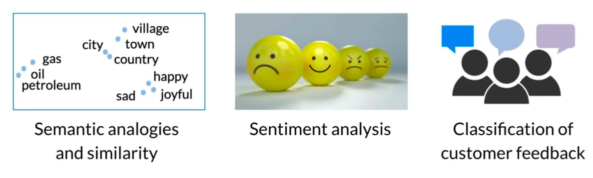
Word embeddings are used in most NLP applications. Whenever we are dealing with text, we first have to find a way to encode the words as numbers. Word embedding are a very common technique that allows we to do so. Here are a few applications of word embeddings that we should be able to implement by the time we complete the specialization.

By the end of this week we will be able to:
- Identify the key concepts of word representations
- Generate word embeddings
- Prepare text for machine learning
- Implement the continuous bag-of-words model
Basic Word Representations
Basic word representations could be classified into the following:
- Integers
- One-hot vectors
- Word embeddings
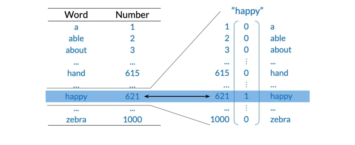
To the left, we have an example where we use integers to represent a word. The issue there is that there is no reason why one word corresponds to a bigger number than another. To fix this problem we introduce one hot vectors (diagram on the right). To implement one hot vectors, we have to initialize a vector of zeros of dimension V and then put a 1 in the index corresponding to the word we are representing.
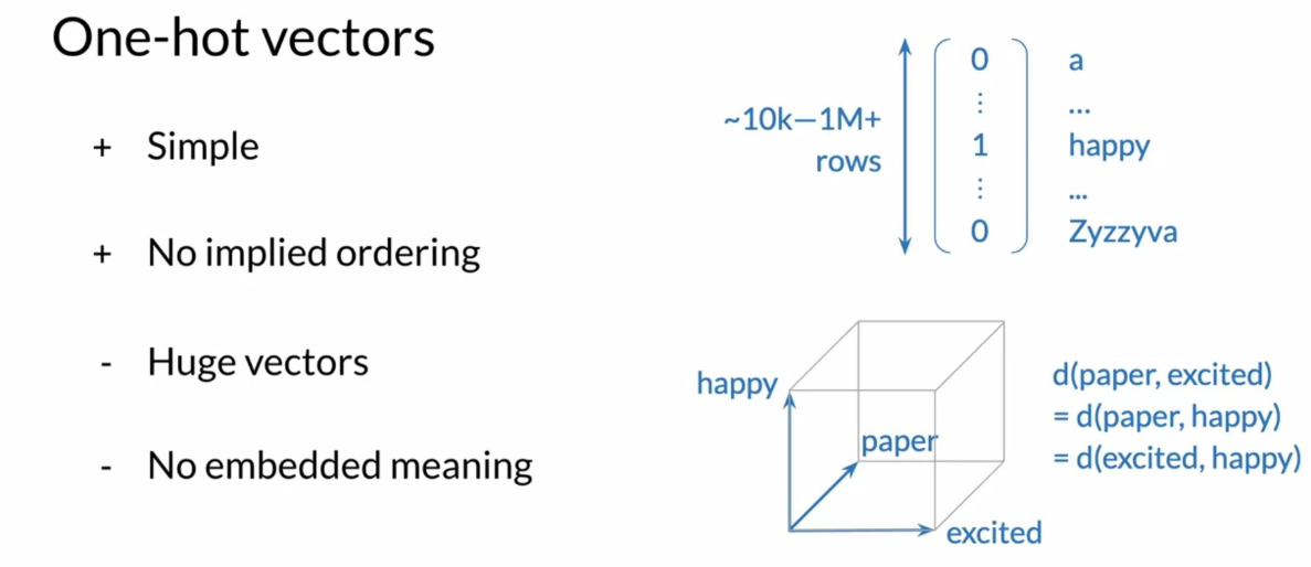
The pros of one-hot vectors: simple and require no implied ordering. The cons of one-hot vectors: huge and encode no meaning.
Word Embeddings
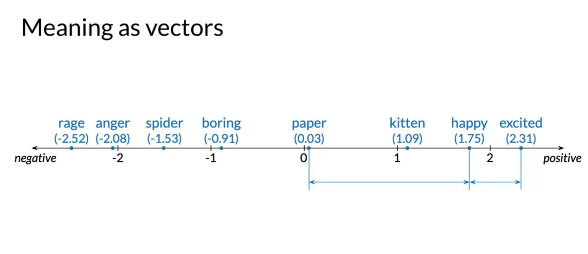
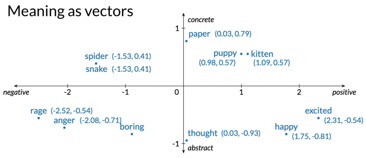
From the plot above, we can see that when encoding a word in 2D, similar words tend to be found next to each other. Perhaps the first coordinate represents whether a word is positive or negative. The second coordinate tell we whether the word is abstract or concrete. This is just an example, in the real world we will find embeddings with hundreds of dimensions. We can think of each coordinate as a number telling we something about the word.
The pros:
- Low dimensions (less than V)
- Allow we to encode meaning
How to Create Word Embeddings?
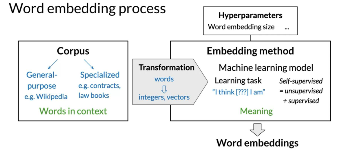
To create word embeddings we always need a corpus of text, and an embedding method.
The context of a word tells we what type of words tend to occur near that specific word. The context is important as this is what will give meaning to each word embedding.
Embeddings There are many types of possible methods that allow we to learn the word embeddings. The machine learning model performs a learning task, and the main by-products of this task are the word embeddings. The task could be to learn to predict a word based on the surrounding words in a sentence of the corpus, as in the case of the continuous bag-of-words.
The task is self-supervised: it is both unsupervised in the sense that the input data — the corpus — is unlabelled, and supervised in the sense that the data itself provides the necessary context which would ordinarily make up the labels.
When training word vectors, there are some parameters we need to tune. (i.e. the dimension of the word vector)
Word Embedding Methods
Classical Methods
- word2vec (Google, 2013)
- Continuous bag-of-words (CBOW): the model learns to predict the center word given some context words.
- Continuous skip-gram / Skip-gram with negative sampling (SGNS): the model learns to predict the words surrounding a given input word.
- Global Vectors (GloVe) (Stanford, 2014): factorizes the logarithm of the corpus’s word co-occurrence matrix, similar to the count matrix you’ve used before.
- fastText (Facebook, 2016): based on the skip-gram model and takes into account the structure of words by representing words as an n-gram of characters. It supports out-of-vocabulary (OOV) words.
Deep learning, contextual embeddings
In these more advanced models, words have different embeddings depending on their context. We can download pre-trained embeddings for the following models.
- BERT (Google, 2018):
- ELMo (Allen Institute for AI, 2018)
- GPT-2 (OpenAI, 2018)
Continuous Bag-of-Words Model
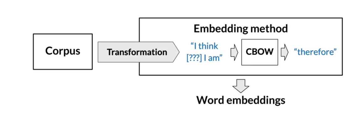
Continuous Bag of Words Model To create word embeddings, we need a corpus and a learning algorithm. The by-product of this task would be a set of word embeddings. In the case of the continuous bag-of-words model, the objective of the task is to predict a missing word based on the surrounding words.
Here is a visualization that shows we how the models works.
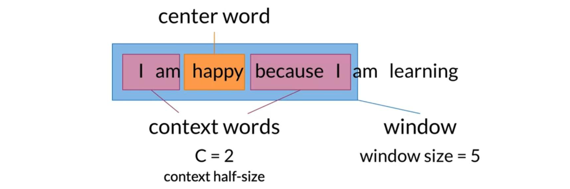
As we can see, the window size in the image above is 5. The context size, C, is 2. C usually tells we how many words before or after the center word the model will use to make the prediction. Here is another visualization that shows an overview of the model.
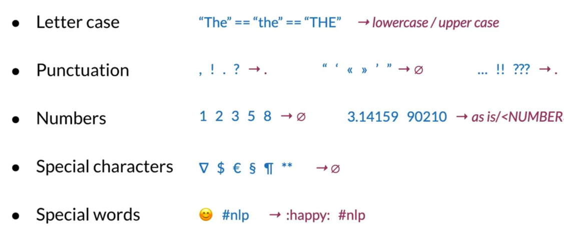
Cleaning and Tokenization
Before implementing any natural language processing algorithm, we might want to clean the data and tokenize it. Here are a few things to keep track of when handling your data.
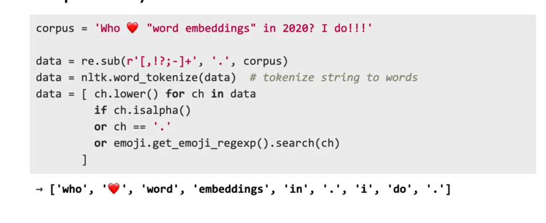
We can clean data using python as follows:
We can add as many conditions as we want in the lines corresponding to the green rectangle above.
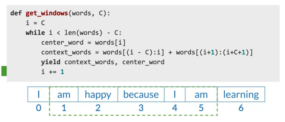
Sliding Window of words in Python
The code above shows we a function which takes in two parameters.
Words: a list of words.
C: the context size.
We first start by setting i to C. Then we single out the center_word, and the context_words. We then yield those and increment i.
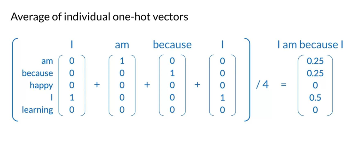
Transforming Words into Vectors
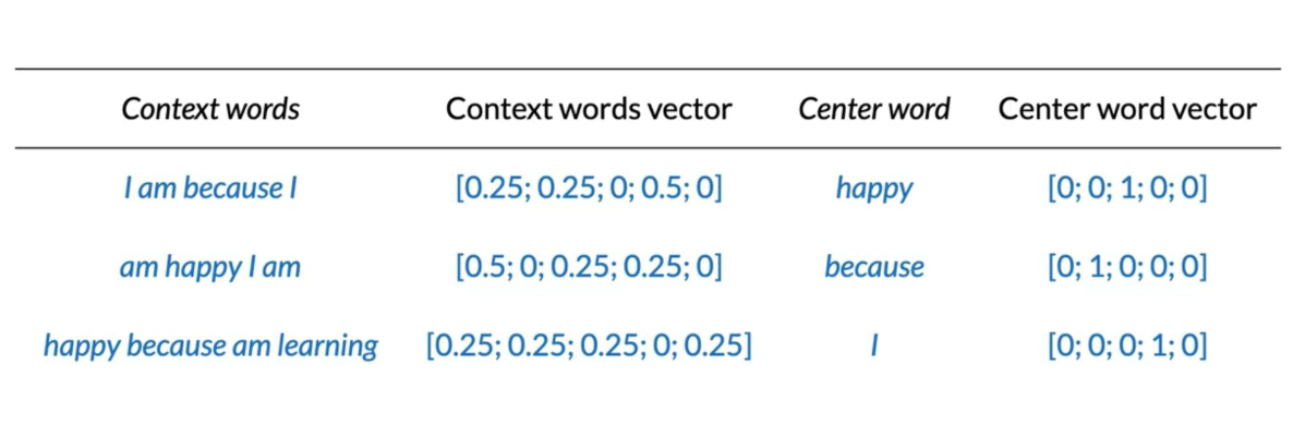
As we can see, we started with one-hot vectors for the context words and and we transform them into a single vector by taking an average. As a result we end up having the following vectors that we can use for your training.
Lecture Notebook - Data Preparation
Architecture of the CBOW Model
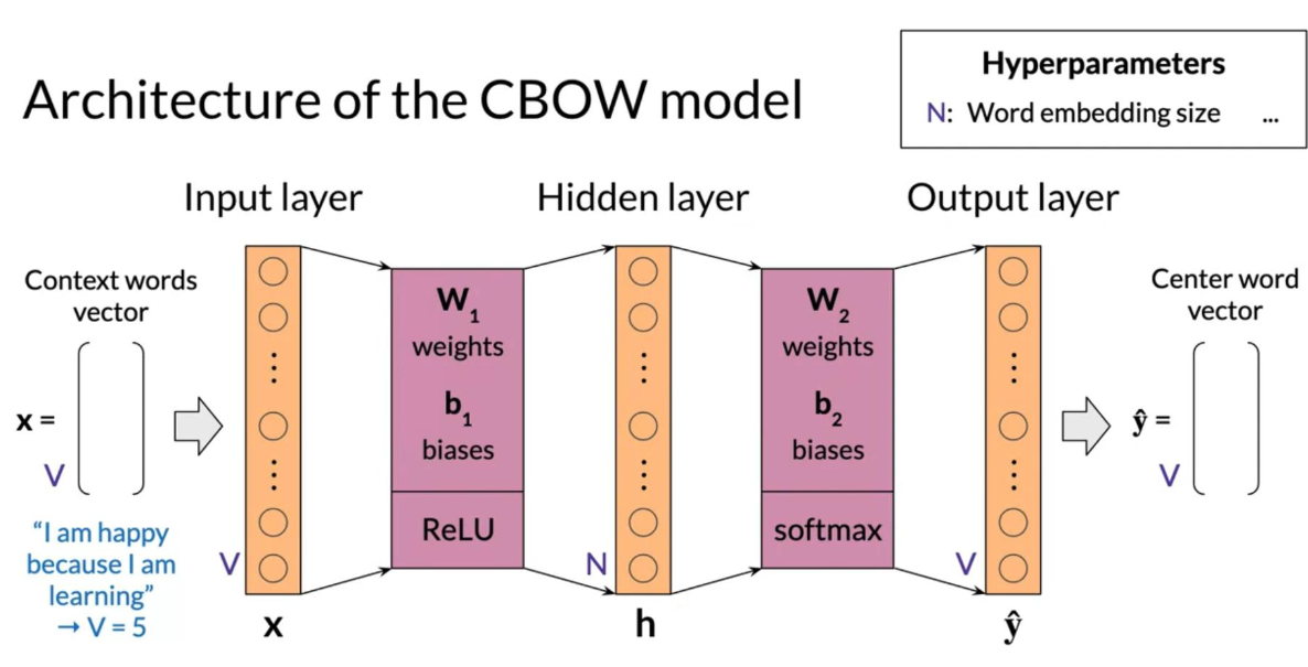
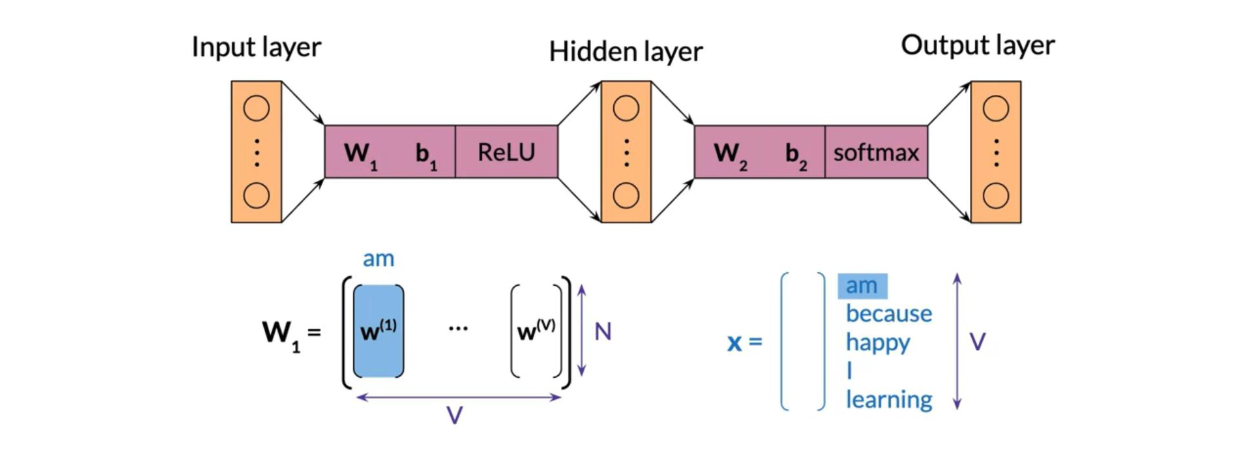
The architecture for the CBOW model could be described as follows
We have an input, X, which is the average of all context vectors. We then multiply it by W_1 and add b1. The result goes through a ReLU function to give we your hidden layer. That layer is then multiplied by W_2 and we add b_2. The result goes through a softmax which gives we a distribution over V, vocabulary words. We pick the vocabulary word that corresponds to the arg-max of the output.
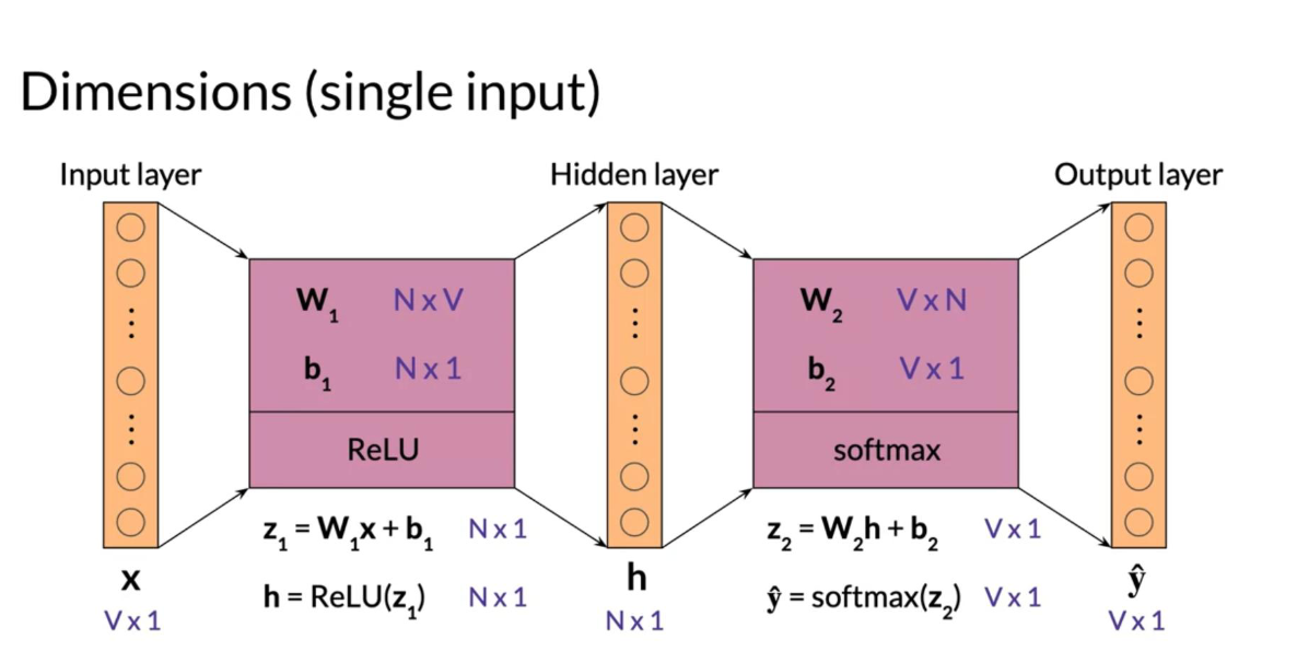
Architecture of the CBOW Model: Dimensions
The equations for the previous model are:
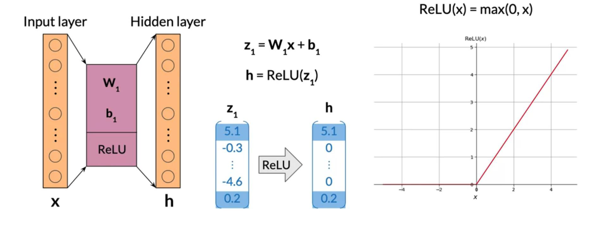
z_1 = W_1 x + b_1
h = ReLU(z_1)
z_2 = W_2 h + b_2
\hat{y} = softmax(z_2)
Here, we can see the dimensions:
Make sure we go through the matrix multiplications and understand why the dimensions make sense.
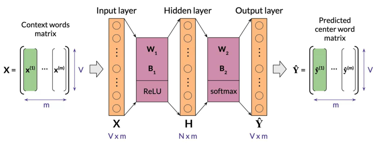
Architecture of the CBOW Model: Dimensions 2
When dealing with batch input, we can stack the examples as columns. We can then proceed to multiply the matrices as follows:
In the diagram above, we can see the dimensions of each matrix. Note that your \hat{Y} is of dimension V by m. Each column is the prediction of the column corresponding to the context words. So the first column in \hat{Y} is the prediction corresponding to the first column of X.
Architecture of the CBOW Model: Activation Functions
ReLU funciton
The rectified linear unit (ReLU), is one of the most popular activation functions. When we feed a vector, namely x, into a ReLU function. We end up taking x=max(0,x). This is a drawing that shows ReLU.
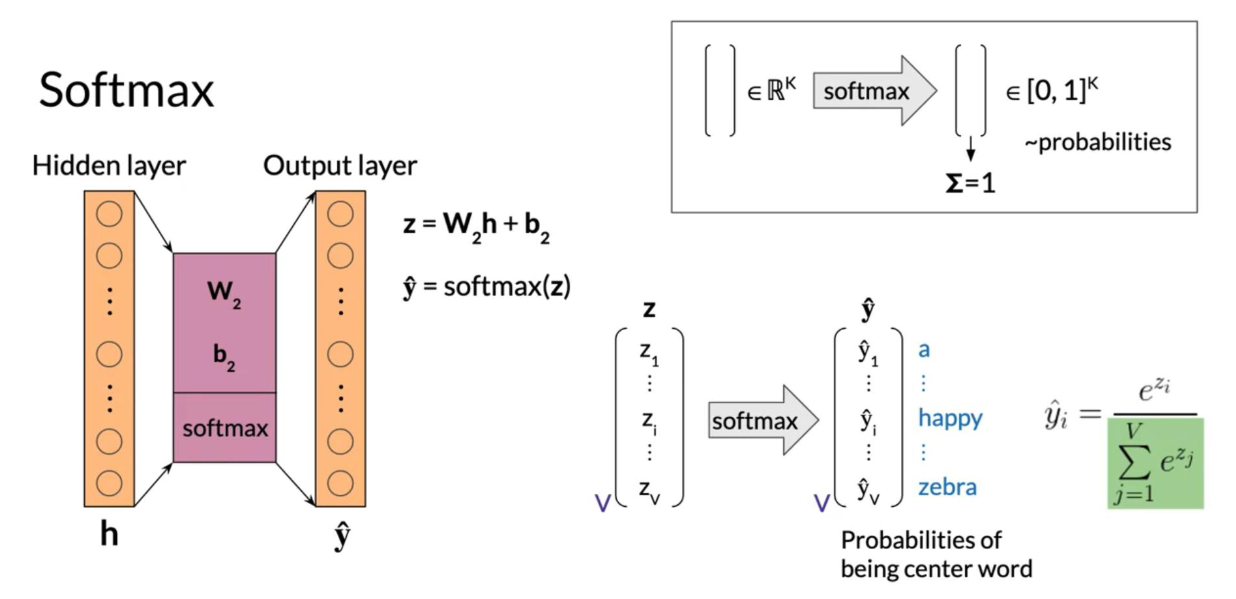
Softmax function
The softmax function takes a vector and transforms it into a probability distribution. For example, given the following vector z, we can transform it into a probability distribution as follows.
As we can see, we can compute:
\hat{y} = \frac{e^{z_i}}{\sum_{j=1}^V e^{z_j}}
Lecture Notebook - Intro to CBOW model
Training a CBOW Model: Cost Function
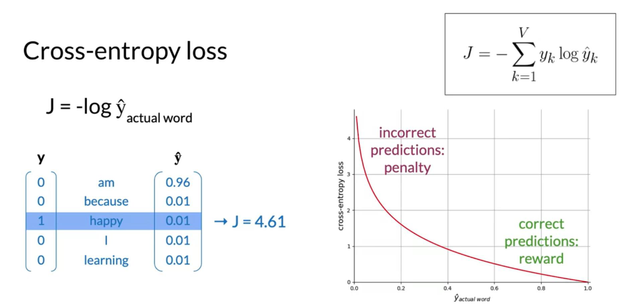
The cost function for the CBOW model is a cross-entropy loss defined as:
J = -\sum_{k=1}^V y_k log(\hat{y}_k) \tag{1}
Here is an example where we use the equation above.
Why is the cost 4.61 in the example above?
Training a CBOW Model: Forward Propagation
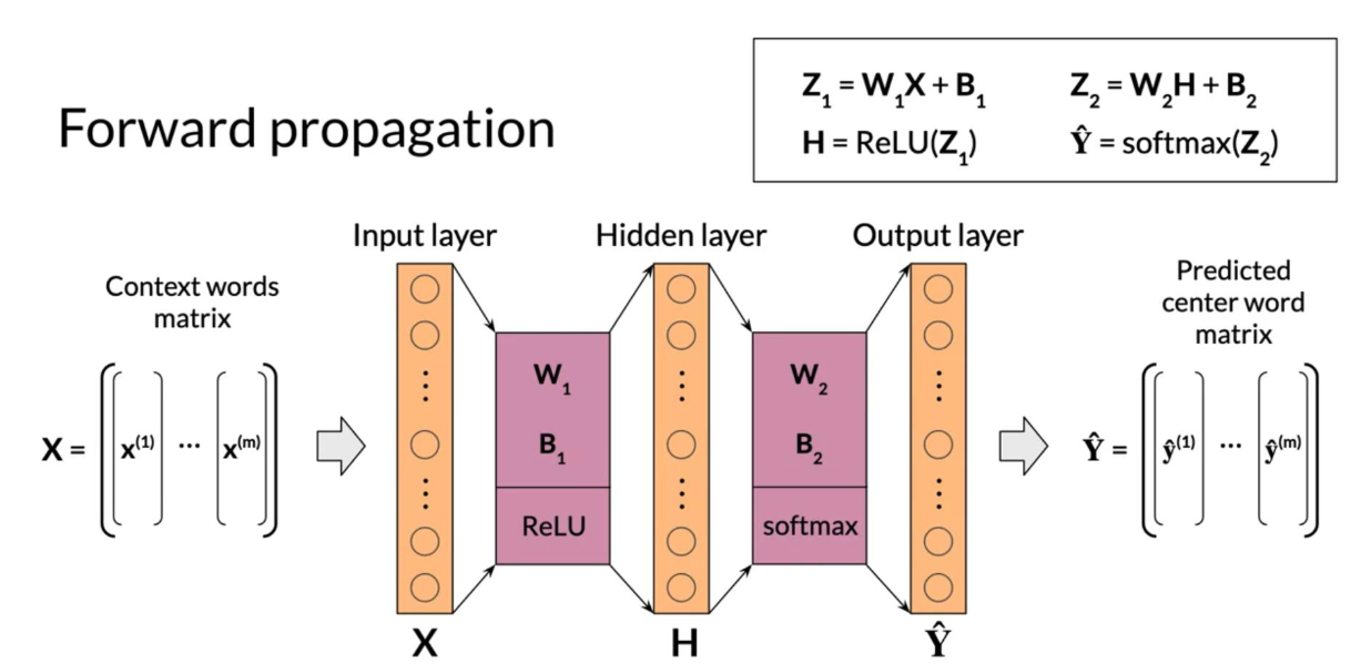
Training a CBOW Model: Forward Propagation Forward propagation is defined as:
Z_1 = W_1 X + B_1
H = ReLU(Z_1)
Z_2 = W_2 H + B_2
\hat{Y} = softmax(Z_2)
In the image below we start from the left and we forward propagate all the way to the right.
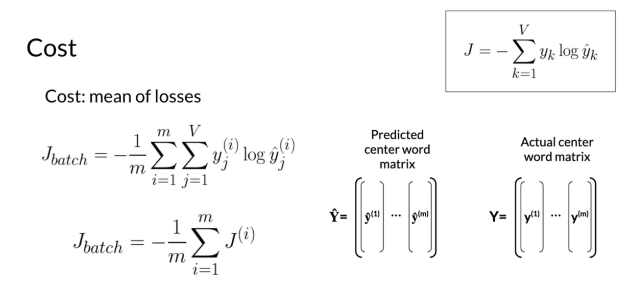
To calculate the loss of a batch, we have to compute the following:
J_{batch} = -\frac{1}{m} \sum_{i=1}^m \sum_{j=1}^V y_j(i) log(\hat{y}^j(i))
Given, your predicted center word matrix, and actual center word matrix, we can compute the loss.
Training a CBOW Model: Backpropagation and Gradient Descent
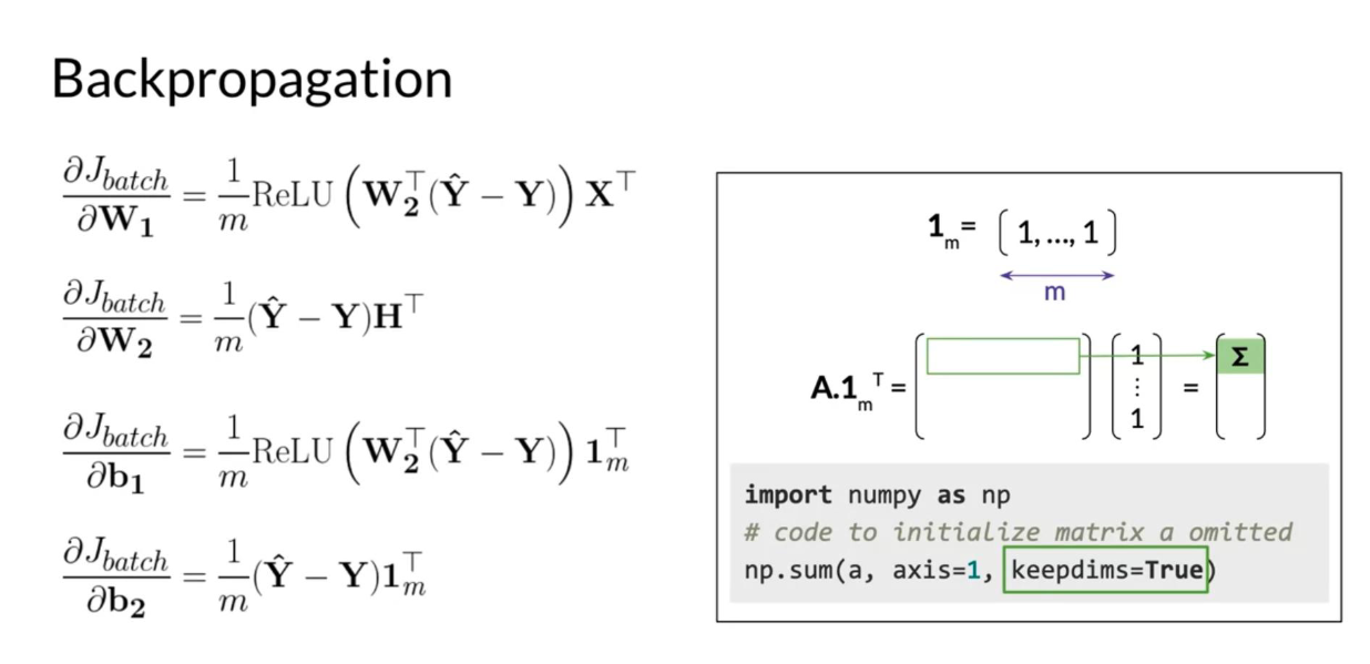
Training a CBOW Model: Backpropagation and Gradient Descent Backpropagation: calculate partial derivatives of cost with respect to weights and biases.
When computing the back-prop in this model, we need to compute the following:
\frac{\partial J_{batch}}{\partial W_1}, \frac{\partial J_{batch}}{\partial W_2}, \frac{\partial J_{batch}}{\partial B_1}, \frac{\partial J_{batch}}{\partial B_2}
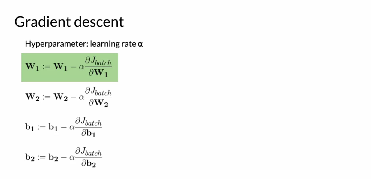
Gradient descent: update weights and biases
Now to update the weights we can iterate as follows:
W_1 := W_1 - \alpha \frac{\partial J_{batch}}{\partial W_1}
W_2 := W_2 - \alpha \frac{\partial J_{batch}}{\partial W_2}
B_1 := B_1 - \alpha \frac{\partial J_{batch}}{\partial B_1}
B_2 := B_2 - \alpha \frac{\partial J_{batch}}{\partial B_2}
A smaller alpha allows for more gradual updates to the weights and biases, whereas a larger number allows for a faster update of the weights. If α is too large, we might not learn anything, if it is too small, your model will take forever to train.
Lecture Notebook - Training the CBOW model
Extracting Word Embedding Vectors
There are two options to extract word embeddings after training the continuous bag of words model. We can use W_1 as follows:
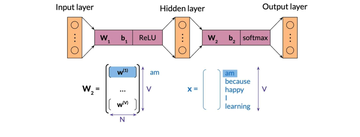
If we were to use W_1, each column will correspond to the embeddings of a specific word. We can also use W_2 as follows:
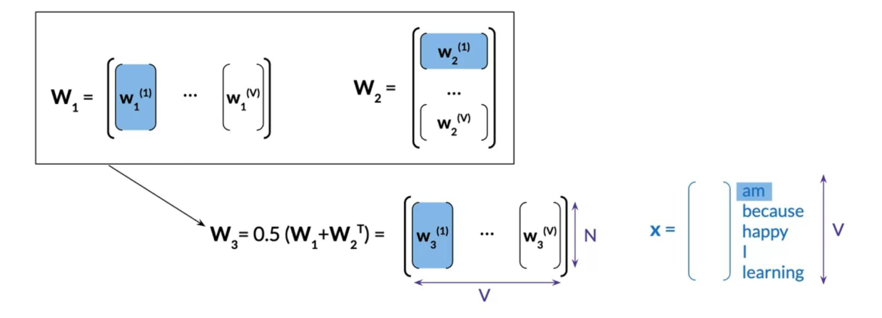
The final option is to take an average of both matrices as follows:
Lecture Notebook - Word Embeddings
Lecture notebook: Word embeddings step by step
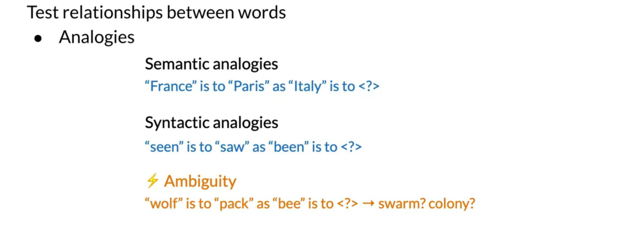
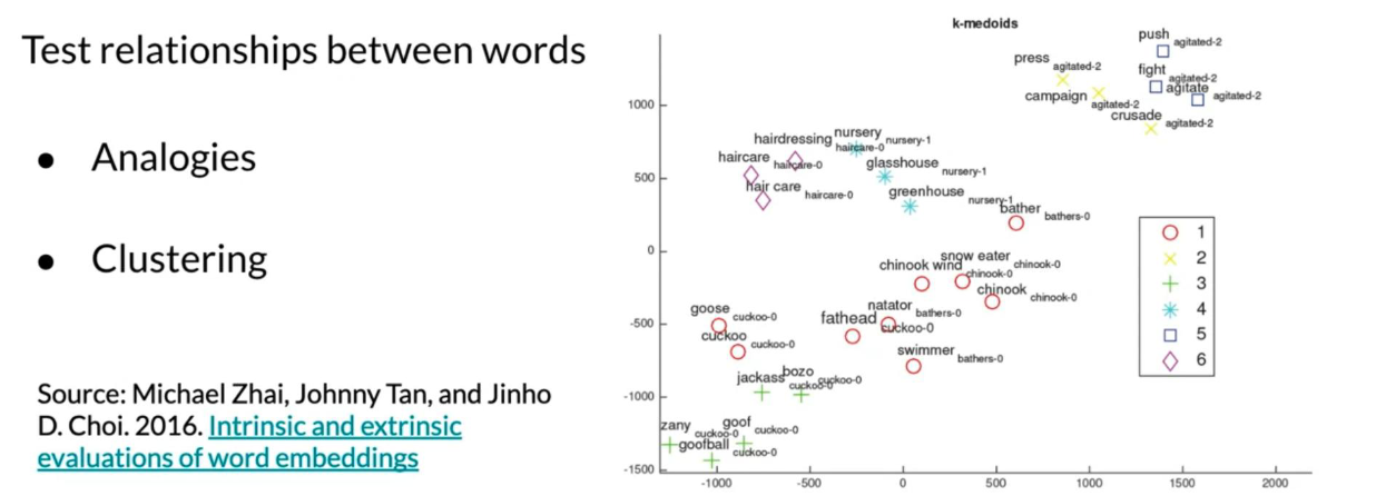
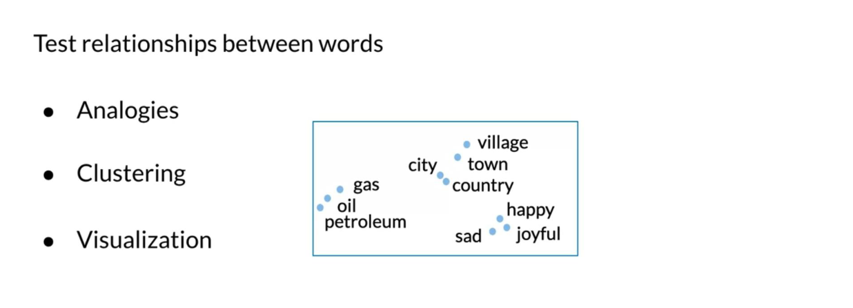
Evaluating Word Embeddings: Intrinsic Evaluation
Intrinsic evaluation allows we to test relationships between words. It allows we to capture semantic analogies as, “France” is to “Paris” as “Italy” is to <?> and also syntactic analogies as “seen” is to “saw” as “been” is to <?>.
Ambiguous cases could be much harder to track:
Here are a few ways that allow to use intrinsic evaluation.
Evaluating Word Embeddings: Extrinsic Evaluation
Extrinsic evaluation tests word embeddings on external tasks like named entity recognition, parts-of-speech tagging, etc.
- Evaluates actual usefulness of embeddings
- Time Consuming
- More difficult to trouble shoot
So now we know both intrinsic and extrinsic evaluation.
Conclusion
This week we learned the following concepts.
- Data preparation
- Word representations
- Continuous bag-of-words model
- Evaluation
We have all the foundations now. From now on, we will start using some advanced AI libraries in the next courses. Congratulations and good luck with the assignment
Citation
@online{bochman2020,
  author = {Bochman, Oren},
  title = {Word Embeddings with Neural Networks},
  date = {2020-10-29},
  url = {https://orenbochman.github.io/notes-nlp/notes/c2w4/},
  langid = {en}
}