Vector Space Models

Figure 1: course banner

Figure 2

Vector Space Models

linear representation

Figure 3: Understanding Vector Space

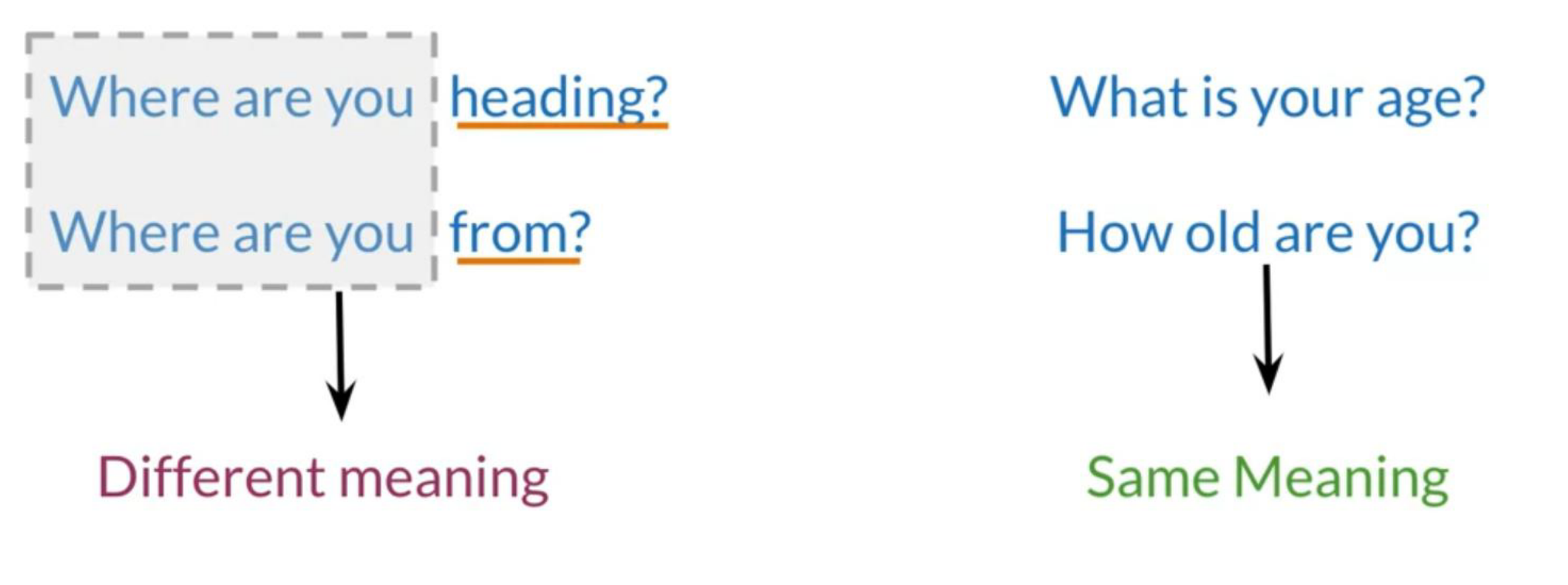
Vector spaces are fundamental in many applications in NLP. If we were to represent a word, document, tweet, or any form of text, we will probably be encoding it as a vector. These vectors are important in tasks like information extraction, machine translation, and chatbots. Vector spaces could also be used to help we identify relationships between words as follows:

• We eat cereal from a bowl
• We buy something and someone else sells it

Distributed Representation

Figure 4: Distributed Representation is A fundamental concept in Linguistics

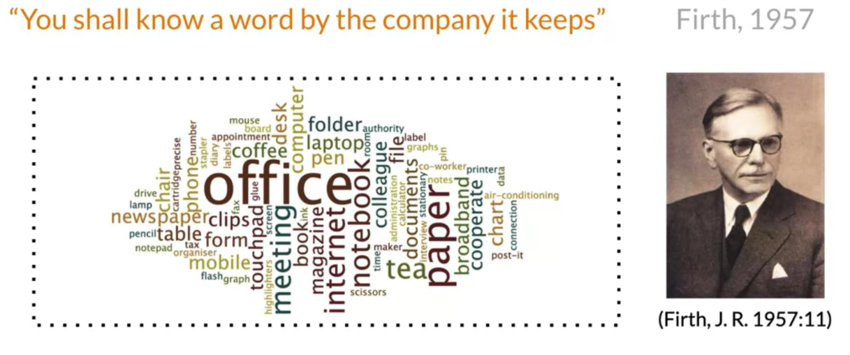
“We shall know a word by the company it keeps”. – J.R. Firth

When we are learning these vectors, we usually make use of the neighboring words to extract meaning and information about the center word. If we were to cluster these vectors together, we will see that adjectives, nouns, verbs, etc. tend to be near one another. Another aspect of the vector space representation, is that synonyms and antonyms are also very close to one another. This is because we can easily interchange them in a sentence and they tend to have similar neighboring words!

linear representation

Figure 5: Some applications of the vector space model in NLP

Word-by-Word and Word By Document

We now delve into constructing vector word representations, based off a co-occurrence matrix. Specifically, depending on the task we are trying to solve, we can choose from several possible designs.

Word by word Design

We will start by exploring the word by word design. Assume that we are trying to come up with a vector that will represent a certain word. One possible design would be to create a matrix where each row and column corresponds to a word in your vocabulary. Then we can iterate over a document and see the number of times each word shows up next each other word. We can keep track of the number in the matrix. In the video I spoke about a parameter K.

We can think of K as the window size for the context which determines if two words are considered adjacent according to Firth’s law.

Word by word design

Figure 6: Word Level aggregation: Creating a word by word vector space using a word by word design

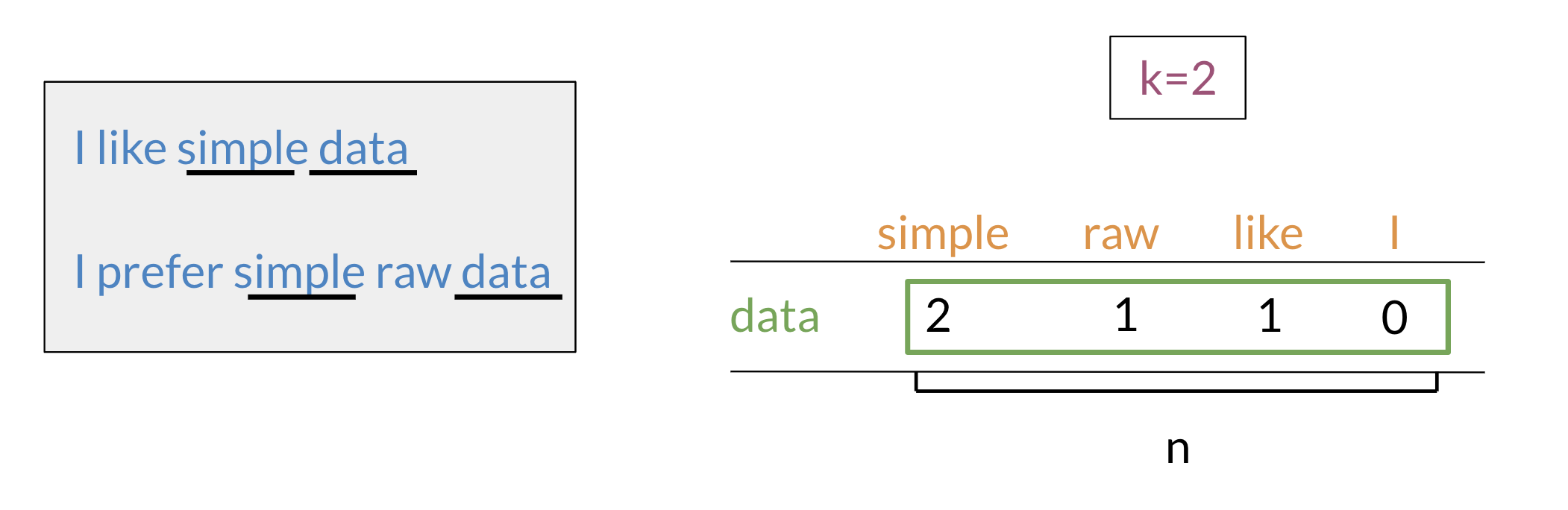
In the example above, we can see how we are keeping track of the number of times words occur together within a certain distance k. At the end, we can represent the word data, as a vector v=[2,1,1,0].

Word by Document Design

We can now apply the same concept and map words to documents. The rows could correspond to words and the columns to documents. The numbers in the matrix correspond to the number of times each word showed up in the document.

Word by document

Figure 7: Document Level aggregation: Creating a document by word vector space using a word by word design

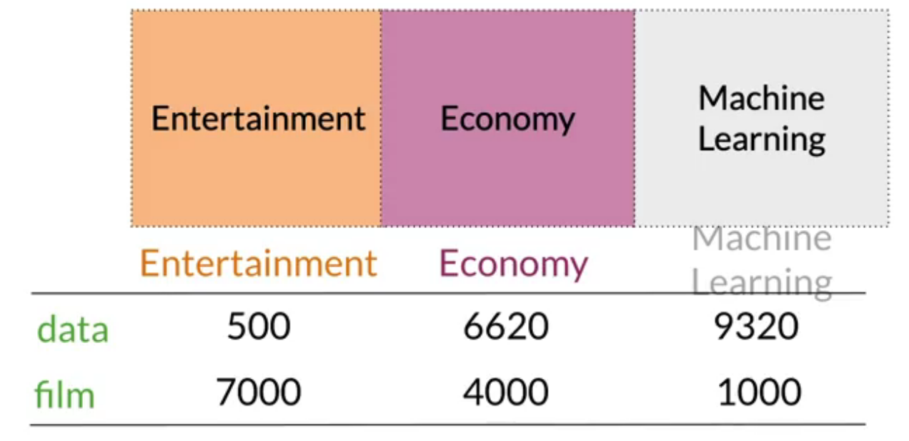
In the example above, we can see how we are keeping track of the number of times words occur together within a certain distance k.

At the end, we can represent the word data, as a vector v = [2, 1, 1, 0].

linear representation

Figure 8: In this slide we see the vector space matrix at the top left, and on the right a plot of the it geometry of two words in three document categories. We can use the angle and the distance between these vectors to understand the similarity between the vectors.

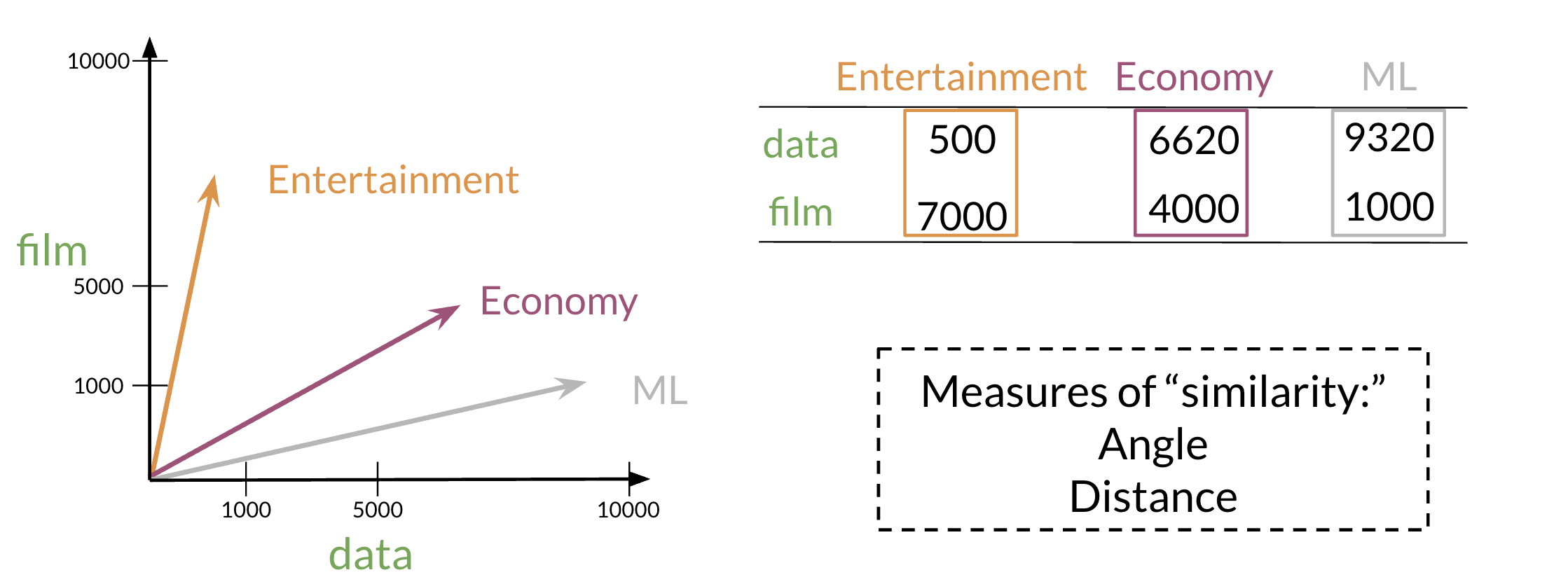
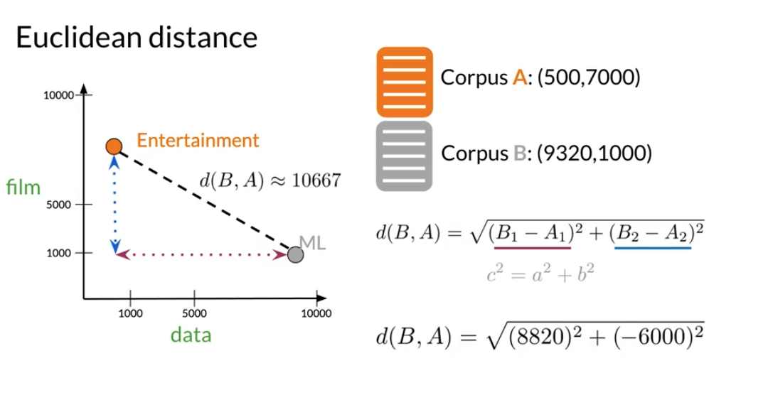
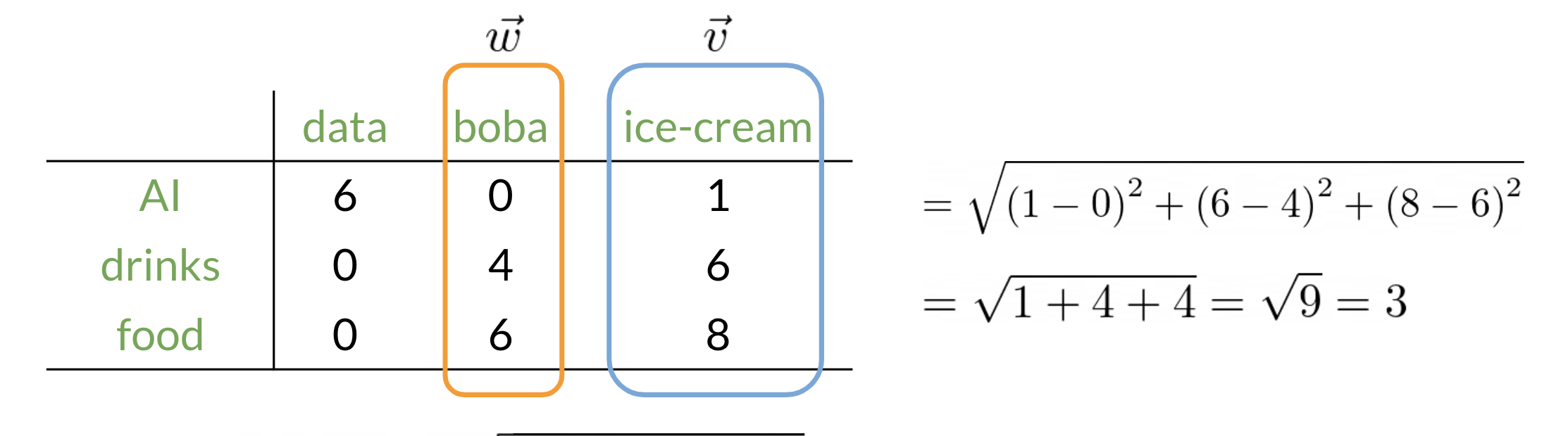
Euclidean Distance

Let us assume that we want to compute the distance between two points: A,B. To do so, we can use the euclidean distance defined as

d(B,A) = \sqrt{\sum_{i=1}^{n} (B_i - A_i)^2} \tag{1}

Euclidean distance

Figure 9: In this slide we see the vector space matrix at the top left, and on the right a plot of the it geometry of two words in three document categories. We can use the angle and the distance between these vectors to understand the similarity between the vectors.

Distance calculation

Figure 10: Calculate the distance between two vectors of dimensional size three.

LAB: Linear algebra in Python with numpy

The Numpy lab

Cosine Similarity Intuition

One of the issues with euclidean distance is that it is not always accurate and sometimes we are not looking for that type of similarity metric. For example, when comparing large documents to smaller ones with euclidean distance one could get an inaccurate result.

Look at the diagram:

Cosine Similarity: Intuition

Figure 11: The cosine similarity is the cosine of the angle between two vectors.

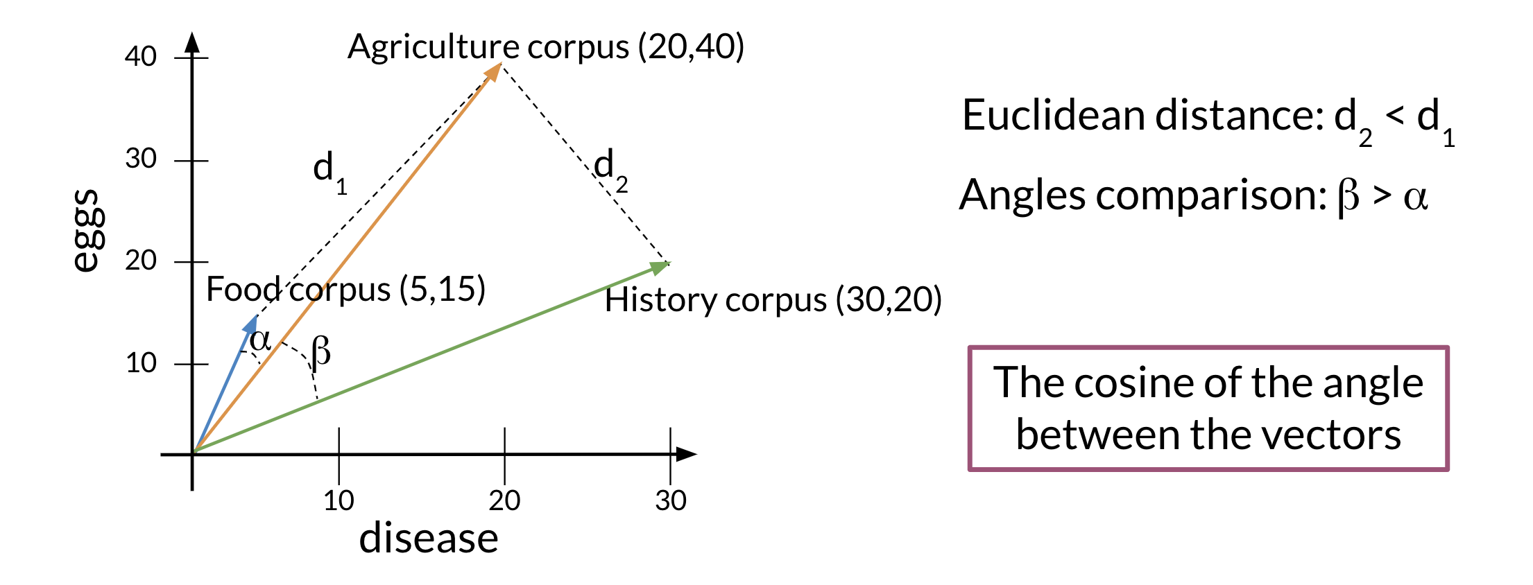
Normally the food corpus and the agriculture corpus are more similar because they have the same proportion of words. However the food corpus is much smaller than the agriculture corpus. To further clarify, although the history corpus and the agriculture corpus are different, they have a smaller euclidean distance. Hence d_2<d_1.

To solve this problem, we look at the cosine between the vectors. This allows us to compare B and α.

Background

Before getting into the cosine similarity function remember that the norm of a vector is defined as:

Norm of a Vector

||\vec{A}|| = \sqrt{\sum_{i=1}^{n} a_i^2} \tag{2}

Dot-product of Two Vectors

The dot product is then defined as:

\vec{A} \cdot \vec{B} = \sum_{i=1}^{n} a_i \cdot b_i \tag{3}

Cosine Similarity

Figure 12: The cosine similarity is the cosine of the angle between two vectors.

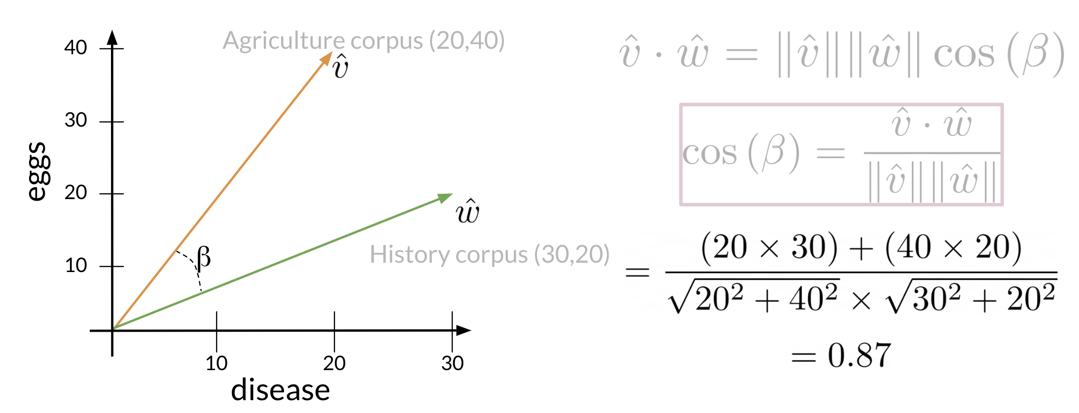
The following cosine similarity equation makes sense:

\cos(\theta) = \frac{\vec{v} \cdot \vec{w}}{||\vec{v}|| \cdot ||\vec{w}||} \tag{4}

Implementation

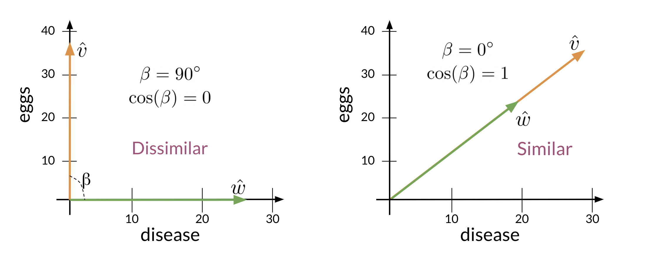
When \vec{v} and \vec{u} are parallel the numerator is equal to the denominator so cos(\beta)=1 thus \angle \beta=0.

On the other hand, the dot product of two orthogonal (perpendicular) vectors is 0. That takes place when \angle \beta=90.

Cosine Similarity Examples

Figure 13: Examples of cosine similarity between similar and dissimilar vectors.

Word Manipulation in Vector Spaces

We can use word vectors to actually extract patterns and identify certain structures in your text. For example:

Word analogy conceptual

Figure 14: Word analogy have a geometric interpretation in vector spaces.

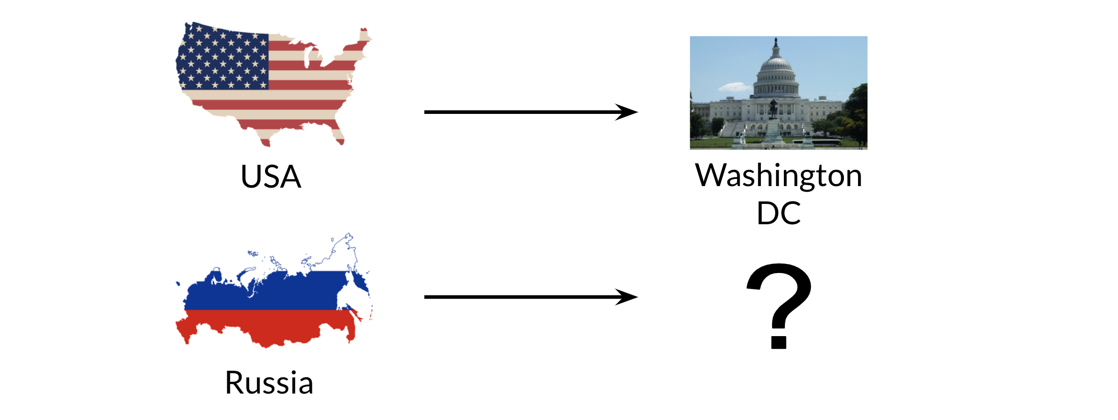
We can use the word vector for Russia, USA, and DC to actually compute a vector that would be very similar to that of Moscow. We can then use cosine similarity of the vector with all the other word vectors we have and we can see that the vector of Moscow is the closest.

Isn’t that goofy?

Word analogy

Figure 15: Some word analogies

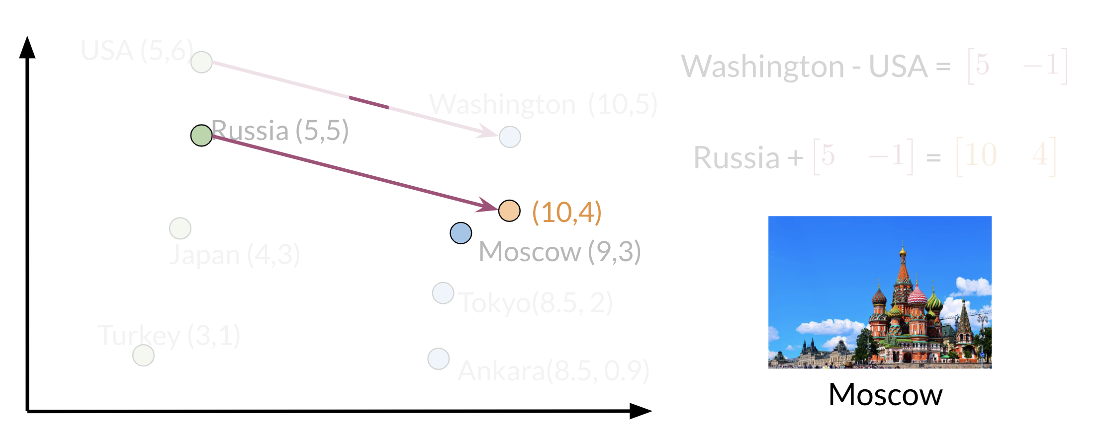
Note that the distance (and direction) between a country and its capital is relatively the same. Hence manipulating word vectors allows we identify patterns in the text.

Lab on Manipulating Word Vectors

The lab

PCA

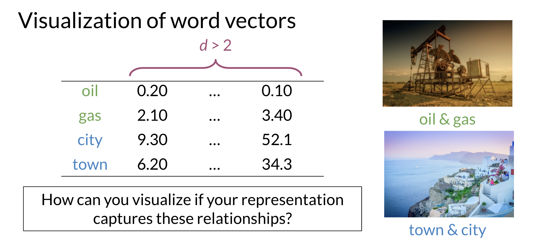
Visualization of Word Vectors

Principal component analysis is an unsupervised learning algorithm which can be used to reduce the dimension of your data. As a result, it allows we to visualize your data. It tries to combine variances across features. Here is a concrete example of PCA:

Word analogy

Figure 16: Some word analogies

Word analogy

Figure 17: Some word analogies

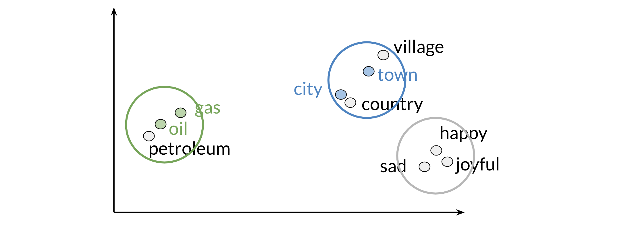
Those are the results of plotting a couple of vectors in two dimensions. Note that words with similar part of speech (POS) tags are next to one another. This is because many of the training algorithms learn words by identifying the neighboring words. Thus, words with similar POS tags tend to be found in similar locations. An interesting insight is that synonyms and antonyms tend to be found next to each other in the plot. Why is that the case?

Implementation

PCA algorithm

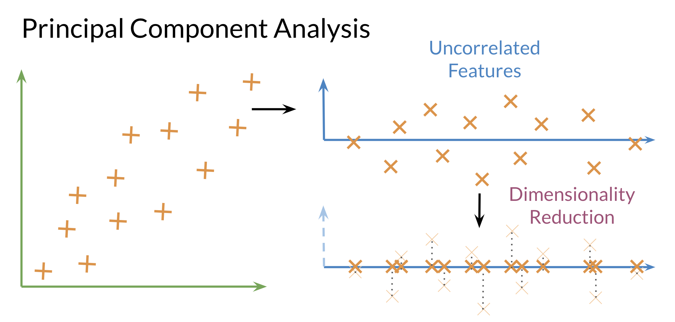
PCA is commonly used to reduce the dimension of your data. Intuitively the model collapses the data across principal components. We can think of the first principal component (in a 2D dataset) as the line where there is the most amount of variance. We can then collapse the data points on that line. Hence we went from 2D to 1D. We can generalize this intuition to several dimensions.

PCA

Figure 18: Some word analogies

Eigenvector

the resulting vectors, also known as the uncorrelated features of your data

Eigenvalue

the amount of information retained by each new feature. We can think of it as the variance in the eigenvector.

Also each eigenvalue has a corresponding eigenvector. The eigenvalue tells we how much variance there is in the eigenvector. Here are the steps required to compute PCA:

PCA

Figure 19: Some word analogies

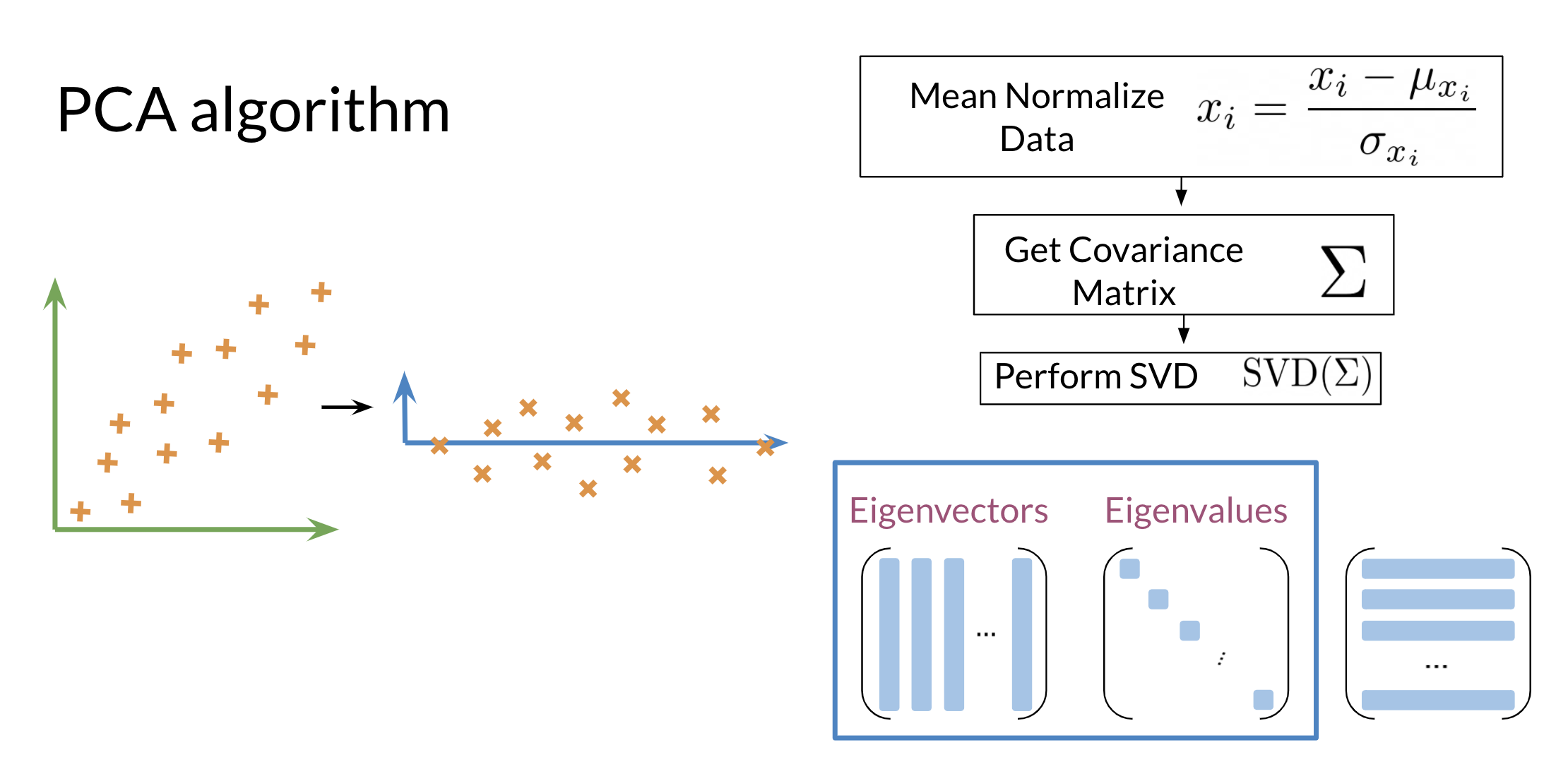
Steps to Compute PCA:

• Mean normalize your data
• Compute the covariance matrix
• Compute SVD on your covariance matrix. This returns [USV]=svd(Σ) . The three matrices U, S, V are drawn above. U is labelled with eigenvectors, and S is labelled with eigenvalues.
• We can then use the first n columns of vector U, to get your new data by multiplying XU[:,0:n].

Putting It Together with Code

import numpy as np 

def PCA(X , num_components):
  # center data around the mean
  X_meaned = X - np.mean(X , axis = 0) 
  # calculate the covariance matrix   
  cov_mat = np.cov(X_meaned , rowvar = False) 
  # compute an uncorrelated feature basis (eigen vectors) 
  eigen_values , eigen_vectors = np.linalg.eigh(cov_mat)
  # sort the new basis by decreasing eigen values (variance) 
  sorted_index = np.argsort(eigen_values)[::-1] 
  sorted_eigenvalue = eigen_values[sorted_index] 
  sorted_eigenvectors = eigen_vectors[:,sorted_index] 
  # by subseting the most leading features  
  eigenvector_subset = sorted_eigenvectors[:,0:num_components] 
  #Step-6 
  X_reduced = np.dot(eigenvector_subset.transpose() ,     
                   X_meaned.transpose() ).transpose() 
  return X_reduced 

Lab on PCA

PCA lab

Document As a Vector

Resources

• Alex Williams - Everything we did and didn’t know about PCA
• Udell et al. (2015). Generalized Low-Rank Models  arxiv preprint
• Tipping & Bishop (1999). Probabilistic principal component analysis Journal of the Royal Statistical Society: Series B
• Ilin & Raiko (2010) Practical Approaches to Principal Component Analysis in the Presence of Missing Values Journal of Machine Learning Research
• Gordon (2002). Generalized² Linear² Models NIPS
• Cunningham & Ghahramani (2015)  Linear dimensionality reduction: survey, insights, and generalizations Journal of Machine Learning Research
• Burges (2009). Dimension Reduction: A Guided Tour Foundations varia Trends in Machine Learning
• M. Gavish and D. L. Donoho, The Optimal Hard Threshold for Singular Values is \frac{4}{\sqrt{3}} in IEEE Transactions on Information Theory, vol. 60, no. 8, pp. 5040-5053, Aug. 2014, doi: 10.1109/TIT.2014.2323359.
• Thomas P. Minka Automatic choice of dimensionality for PCA Dec. 2000